This article is aimed at anyone who is interested in understanding the details of A/B testing from a Bayesian perspective. It is accompanied by a Python project on Github, which I have named aByes (I know, I could have chosen something different from the anagram of Bayes…) and will give you access to a complete set of tools to do Bayesian A/B testing on conversion rate experiments.
The blog post builds from the works of John K. Kruschke, Chris Stucchio and Evan Miller. I believe it gives a comprehensive and critical view on the subject. More importantly, it gives some practical examples that make use aByes. If you are in a hurry and are only interested in the tool, you can skip the boring part and go directly to the case study section. However, if some definitions are not clear I am afraid you will have to go through some of the boring sections. So get your cup of coffee and keep reading :)
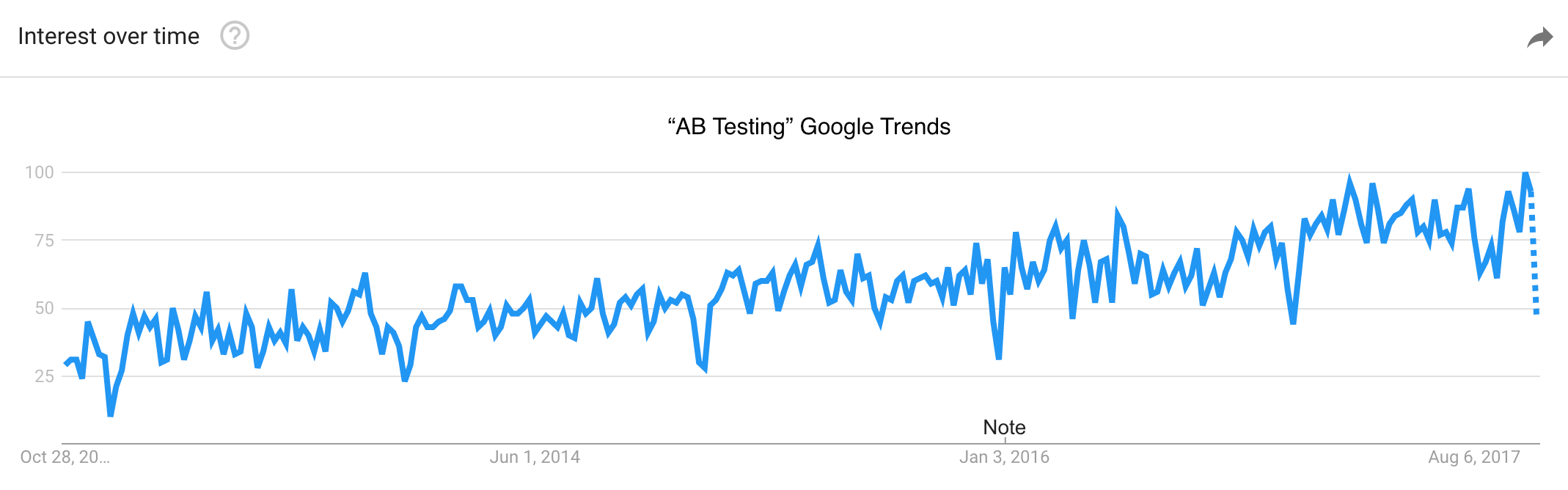
Before starting, it is worth mentioning that the topic of A/B testing has seen increased interest over the past few years (so… well done for reading this blog post!). This is obvious from the figure below, showing how the popularity of the search query “AB Testing” in Google Trends has grown linearly for at least the past five years.
Truth is, every web-company with a big enough basin of users does A/B testing (or, at least, it should). Starting from the big giants like Google, Amazon or Facebook. The general public has learnt (and quickly forgot) about A/B testing when in 2013 Facebook released a paper showing a contagion effect of emotion on its News Feed [1], which generated a wave of indignation across the web (for example, see this article from The Guardian).
For anyone interested in introducing these optimization practices (i.e., A/B testing) in their company, there are commercial tools that can help. Some of the most popular ones are Optimizely and Virtual Website Optimizer (VWO). These two tools follow two different viewpoints for doing inferential statistics: Optimizely uses a Frequentist approach, while VWO uses a Bayesian approach.
Here I am not going to digress on the differences between Frequentism and Bayesianism (personally I don’t have a strong preference against one or the other). From now on, we will simply deep dive into the A/B testing world - as seen by a Bayesian.
The main steps needed for doing Bayesian A/B testing are three:
1. Collect the data for the experiment;
2. Compare the different variants by applying Bayes’ Theorem;
3. Decide whether or not the experiment has reached a statistically significant result and can be stopped.
These three steps are visualized in the flow chart below, which give a more complete view of the different choices that a practitioner needs to make. The meaning of these options (analytic/MCMC solution and ROPE/Expected Loss decision rule) will become clear as you keep reading this blog post.
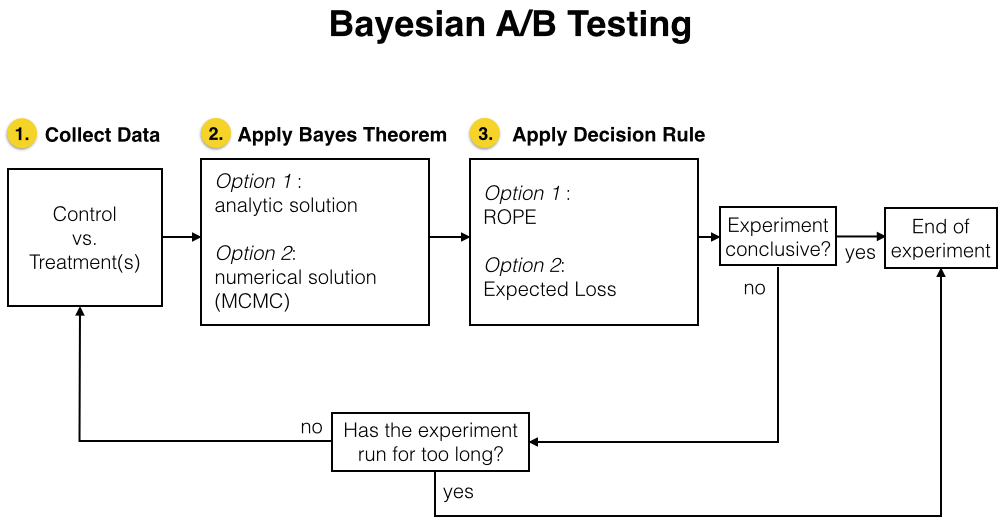
And now, let’s discuss each of these steps individually.
1. Collect the Data
This is the “engineering” step of the lot. As such, I am only going to briefly touch on it.
It is obvious that collecting data is the first thing that should be developed in the experimental pipeline. Users should be randomized in the “A” and “B” buckets (often called the “Control” and “Treatment” buckets). The client (the browser) should send events, typically click events, to a specific endpoint that should be accessible for our analysis. The endpoint could be a database hosted on the backend, or more advanced solutions that are possible with cloud services such as AWS.
If I were to start from scratch I would consider using a backend tool such as Facebook PlanOut for randomizing the users and serving the different variants to the client. I would then use a data warehouse such as Amazon Redshift for storing all the event logs.
It is important to make sure that users are always exposed to the same variant when they access the website during the experiment, otherwise the experiment itself would be invalidated. This requirement can be ensured by using cookies. Alternative solutions are possible if the users can be uniquely identified (for example if they are logged in on the website).
2. Apply Bayes’ theorem
After we begin collecting the data and for each click event we have at least logged the type of event (for example, if it is a click on a “sign in” or on a “register” button), the unique id of the user and the variation in which he/she was bucketed (let’s say A or B), we can start our analysis.
Every time Bayesian methods are applied, it is always useful to write down Bayes’ theorem. After all, it is so simple that it only requires a minimal amount of effort to remember it.
Assume that $H$ is some hypothesis to be tested, typically the parameters of our model (for our purposes, the conversion rates of our A and B buckets), while $\textbf{d}$ is the data collected during our experiment. Then Bayes’ theorem reads
$$\begin{equation}
\mathbb{P}(H|\textbf{d}) = \frac{\mathbb{P}(\textbf{d}|H)\mathbb{P}(H)}{\mathbb{P}(\textbf{d})}
\label{eq:Bayes}
\end{equation}$$
What do the different terms mean?
- $\mathbb{P}(H|\textbf{d})$: posterior distribution. It is the quantity that we are interested in quantifying. It is the probability that some specific hypothesis is true, after having collected the data $\textbf{d}$. In terms of our A/B test reasoning, $H$ will be the set of all the possible outcomes of the test. For example, that the conversion rate for A is better than for B by +0.1%, +0.2%, -0.1%, -0.2%, … and every point in between and beyond. As you can imagine, the set of all possible outcomes is infinite which means that $\mathbb{P}(H|\textbf{d})$ will be represented by a continuous distribution.
- $\mathbb{P}(\textbf{d}|H)$: likelihood function. It represents how likely it is to observe the data we have collected, for a given hypothesis of the model. Again, because $H$ is an infinite set of possibilities $\mathbb{P}(\textbf{d}|H)$ is a continuous distribution.
- $\mathbb{P}(H)$: prior distribution. It encodes our information on the model, before observing the data. For example, we may have prior information (through an AA test) that the average conversion rate for A should be centered around 10% with a standard deviation of 1%. Then, our prior for A would be represented by the appropriate normal distribution. Since we don’t have information on B, our best bet would be to assume that B behaves the same as A. In practical terms, this means that the Python project aByes initialises A and B with the same prior.
- $\mathbb{P}(\textbf{d})$: evidence. It is a measure of how well our model fits the data (how good our model is). For continuous distributions, here is how the evidence can be evaluated: $$\mathbb{P}(\textbf{d})=\int \mathbb{P}(\textbf{d}|H)\mathbb{P}(H)\textrm{d}H.$$ The evidence often involves doing multi-dimensional integrals and is the most difficult term to evaluate.
Normally, it is very easy to calculate the posterior distribution $\mathbb{P}(H|\textbf{d})$ up to its normalizing constant. In other words, it is usually easy to calculate the terms in the numerator of Bayes’ theorem. What is difficult to do is to evaluate the evidence $\mathbb{P}(\textbf{d})$. While we don’t always care about it, in many cases we are actually interested in it. It is only by knowing its normalizing constant that we can make the posterior distribution an actual probability distribution (that integrates to one), which we can then use to calculate any other quantities of interest (usually called “moments” of the distribution function).
Unfortunately, for an arbitraty choice of the prior distribution $\mathbb{P}(H)$ it is normally only possible to calculate the posterior distribution - including its normalizing constant - through numerical calculations. In particular, it is common to use Markov Chain Monte Carlo methods. However, for specific type of models and for specific choices of the prior it turns out that the posterior distribution can be calculated analytically. Luckily, it is possible to do so for the analysis of A/B experiments.
To summarize, for A/B testing we have two possible choices for finding out the posterior distribution: 1. analytic method; 2. numerical method. Let’s discuss them in some detail.
2.1 Option 1: Analytic solution
It is often believed that Bayesian methods require more computational power than Frequentist methods. This is a fairly accurate statement, except that in some cases it is possible to solve the Bayesian problem analytically - making the Bayesian solution on par, in terms of speed, with the Frequentist approach.
In order to be able to solve this problem analytically, the prior distributions have to be chosen carefully depending on the form of the likelihood function. For a standard “conversion rate” A/B test, the likelihood function has a particularly simple form: a Bernoulli distribution.
Likelihood function
Most A/B tests involve comparing conversions for users in the Control bucket vs. users in the Treatment bucket. This means that the data will contain, for each user, whether he/she converted or not during the duration of the experiment, like so:
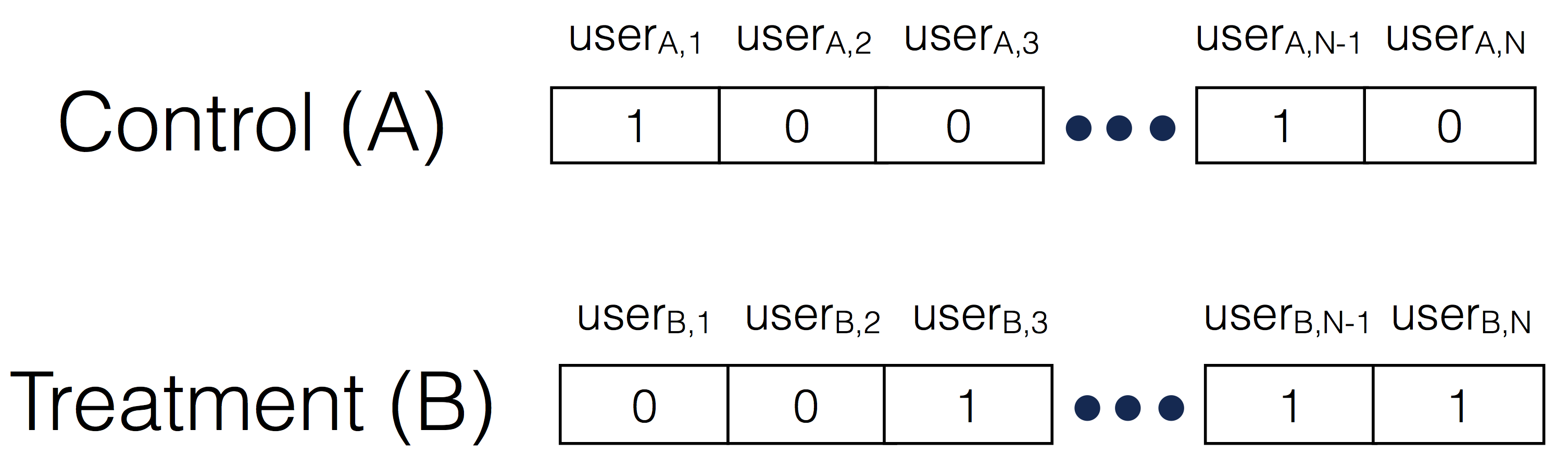
This distribution of ones and zeros has a name: it is a Bernoulli distribution.
Now let’s call the two arrays of binary values as $\textbf{d}_A$ for the Control group and $\textbf{d}_B$ for the Treatment group. Furthermore, let’s say that the Control group has a probability $p_A$ of converting, while the Treatment group has a probability $p_B$ of doing so. Then, the joint likelihood $\mathbb{P}(\textbf{d}|H)$ that enters into Bayes’ theorem can be evaluated as
$$\begin{equation} \mathbb{P}(\textbf{d}|H)=\mathbb{P}(\textbf{d}_A,\textbf{d}_B|p_A,p_B)=\mathbb{P}(\textbf{d}_A|p_A)\mathbb{P}(\textbf{d}_B|p_B)=p_A^{c_A}(1-p_A)^{n_A-c_A}p_B^{c_B}(1-p_B)^{n_B-c_B} \label{eq:likelihood} \end{equation}$$
where we have assumed that the results in the A and B buckets are independent. The quantity in eq. (\ref{eq:likelihood}) represents the probability of observing the data $\textbf{d}_A$ and $\textbf{d}_B$, assuming that the probability of converting are $p_A$ and $p_B$.
Choosing the priors
For specific distributions of the likelihood it is possible to find specific forms of the priors that make the subsequent evaluation of Bayes’ theorem very simple. For the purpose of A/B testing, given the expression (\ref{eq:likelihood}) this “specific form” of the prior is represented by the Beta distribution, which is a continuous distribution defined as a function of $0\leq x \leq 1$ with parameters $\alpha>0$ and $\beta>0$:
$$\begin{equation} \textrm{f}(x; \alpha, \beta) = \frac{x^{\alpha - 1}(1-x)^{\beta-1}}{B(\alpha,\beta)} \label{eq:prior} \end{equation}$$
where
$$B(\alpha,\beta) = \frac{\Gamma(\alpha)\Gamma(\beta)}{\Gamma(\alpha + \beta)},$$
in which $\Gamma$ is the Gamma function.
This will sound rather obscure, but the point is that given our choice of the prior eq. (\ref{eq:prior}) it turns out that the posterior distribution is also a Beta distribution! Because the prior and posterior distributions belong to the same family of Beta distributions, the prior of eq. (\ref{eq:prior}) is called a conjugate prior of the likelihood function eq. (\ref{eq:likelihood}).
We will see just below the exact expression of the posterior distribution.
Finding the posterior distribution
Given our expressions for the likelihood eq. (\ref{eq:likelihood}) and for the priors eq. (\ref{eq:prior}), it is possible to show that the posterior distribution has the following form:
$$\begin{equation} \bbox[lightblue,5px,border:2px solid red]{ \mathbb{P}(H|\textbf{d}) = f(x;\alpha + c_A, \beta + (n_A - c_A))f(x;\alpha + c_B, \beta + (n_B - c_B)) } \label{eq:posterior_analytic} \end{equation}$$
We will see in a moment that this expression agrees perfectly well with the numerical solution (or, rather, the numerical solution agrees with the analytic one!).
2.2 Option 2: Numerical solution
I have fairly extensively talked about pyMC3 in my previous blog post on Bayesian changepoint detection. But fear not, dear reader, there is no need to go through that lengthy blog post to understand how to use pyMC3 for A/B testing. In fact, there is already a pretty good discussion on CrossValidated that has partially inspired this paragraph.
To optimize your learning time, the best thing to do is to look at a Python example. I invite you to copy-paste the code below in a Jupyter notebook and see how the solution looks like.
1 | import numpy as np |
You will see something like this:
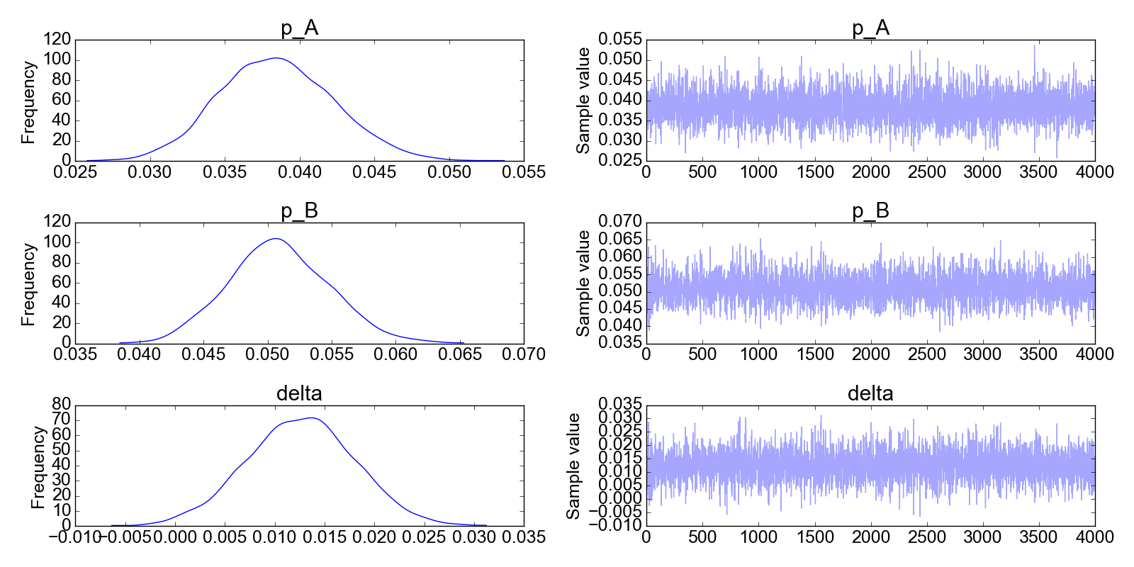
What is this plot telling us? We should first look at the right column. These are the results of the MCMC iterations. The first iterations have been filtered out, that’s where you would see that the algorithm has not yet converged. Instead, in all the plots on the right column you can see that the MCMC solution does not change much, it fluctuates around a mean value. In other words, we can confidently say that the algorithm has converged to its stationary solution (the posterior distribution) and is now randomly sampling from the posterior distribution.
Now, what about the left column? These are simply the histograms of the data in the right column. If, as discussed, we believe the data on the right are all representative of the posterior distribution (i.e., the MCMC algorithm has converged) then these histograms are the answers to our problem: the posterior distribution of the model parameters $p_A, p_B$ and $\Delta$.
Here is the problem that the Python code above solves: suppose that we do an A/B test in which we look at conversion rates. So it happens that the true probability of conversion for the A group is pA_true=0.04 and the one for the B group is pB_true=0.05.
We obviously don’t know what these true probabilities of conversion are, which is the reason for doing an A/B test in the first place… Okay, so let’s say that we collect data for 2500 unique users in the A group and 1750 in the B group. Let’s say that we are completely in the dark at the beginning, so we choose a uniform prior distribution for both groups.
As explained in the paragraph 2.1, the likelihoods are Bernoulli distributions and this is how I have modeled them in pyMC3.
Note that delta is the distribution of the difference in the mean between group A and group B. Line 22 in the code above is actually redundant, as delta could be simply calculated from the trace of p_A and p_B. To convince yourself that this is the case, you can plot two histograms from the commands plt.hist(trace[‘delta’],bins=100) and plt.hist(trace[‘p_B’] - trace[‘p_A’],bins=100): you will observe that the two histograms are identical.
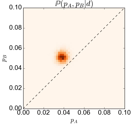
Now… given the information we have how can we actually find out the joint posterior distribution $\mathbb{P}(H|\textbf{d})=\mathbb{P}(p_A,p_B|\textbf{d})$, which represents the left-hand-side in Bayes’ theorem? Although it is not really needed to calculate it, we can just make a two-dimensional histogram of the traces for pA and pB, like so:
1 | matplotlib.rc('font', size=18) |
with the result displayed in the following figure:
2.3 Analytic vs. Numerical Solution
The analytic and numerical solutions have both their advantages and disadvantages. The former is fast and stable. The latter is more flexible, in that it allows for any choice of the prior distribution. However the algorithm is much slower and it requires some extra care such as making sure that the numerical solution has reached convergence.
Overall, I think it makes a lot of sense to use the analytic solution for A/B testing on conversion rates. Even in cases in which we would want to use a specific prior for various reasons (for example after an A/A test, the results of which could be used as priors for a subsequent A/B test), the beta distribution would be flexible enough to be able to “fit” most distributions.
Here I am going to show how the analytic expression for the posterior eq. (\ref{eq:posterior_analytic}) and the numerical MCMC solutions agree. This gives us confidence that either of these methods, as described in this blog post, can be chosen.
The case I am going to discuss is the following. Suppose we start an A/B experiment on conversion rates. The prior distributions for both groups are based on a previous AA experiment and are best fitted by a Beta distribution with $\alpha=3$ and $\beta=10$. We start the experiment and we gather data from 200 users in group A and 200 users also in group B. For this particular case, the data are sampled from a distribution with the (unknown) true conversion probabilities of 0.05 and 0.07 for groups A and B, respectively. The experimental data show 5 conversions out of 200 for group A and 17 conversions out of 200 for group B. Given these data, how do the analytic and numerical solutions look like?
First of all, in order to find the analytic solution we should apply eq. (\ref{eq:posterior_analytic}) with parameters $\alpha=3$, $\beta=10$, $c_A=5$, $n_A=200$, $c_B=17$, $n_B=200$.
It turns out that the posterior distributions agrees very well, as expected (and hoped for). The figure below shows the prior distribution of the conversion rate for the two groups as a dotted line (same prior for the two groups). The red and blue lines, both continuous and broken, show that the pyMC3 solution agress very well with the theoretical one.
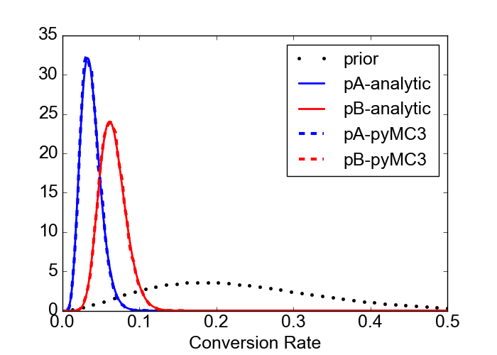
Here is the code used to generate this figure:
1 | from scipy.stats import beta |
At this point we can assume that, either analytically or numerically, we have found our posterior distribution. Okay… now what? Well, we need to apply a decision rule that will tell us whether we have a winner or not. Aren’t you curious to see how this works? Me too!
3. Apply Decision Rule
The third step in our flowchart above consists in applying a decision rule to our analyis: is our experiment conclusive? If so, who is the winner?
To answer this question, it is worth pointing out that Bayesian statistics is much less standardized than Frequentist statistics. Not just because Bayesian statistics is still fairly “young” but also very much because of its richness: Bayesian statistics gives us full access to the distribution of the parameters of interest. This means that there are potentially many different ways of making inference from our data. Nevertheless, the methods will probably become more and more standardized over time.
In terms of A/B testing, there seem to be two main approaches for decision making. The first one is based on the paper by John Kruschke at Indiana University, called “Bayesian estimation supersedes the t test” [2]. It is often cited as the BEST paper (yes, that’s called good marketing strategy ;) ). The decision rule used in this paper is based on the concept of Region Of Practical Equivalence (ROPE) that I discuss in Section 3.1.
The other possible route is the one that makes use of the concept of an Expected Loss. It has been proposed by Chris Stucchio [2] and I discuss it in Section 3.2.
3.1 Option 1: Region Of Practical Equivalence (ROPE) Method
In order to understand this decision rule we need to define the concepts of High Posterior Density Interval (HPD) and Region of Practical Equivalence (ROPE).
3.1.1 High Posterior Density Interval (HPD)
First, let me define the HPD in a formal way before looking at what it means in practice. Here I am borrowing the definition from a nice presentation made available by David Hitchcock [4].
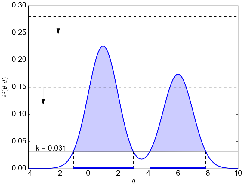
Definition of HPD.
A $100\alpha\%$ HPD region for the parameter $\theta$ is a subset $\mathcal{C}$ of all the possible values of $\theta$ defined by$$\mathcal{C} = {\theta : \mathbb{P}(\theta|\textbf{d}) \geq k}$$
where k is the largest number such that
$$\int_{k\in \mathcal{C}} \mathbb{P}(\theta|\textbf{d}) \textrm{d}\theta = \alpha .$$

Example.
Assume we are looking for the 95% HPD, which means we take $\alpha=0.95$. To find out the 95% HPD for the distribution in the figure below, we do like this: we start with an horizontal line above the maximum. We then start lowering it and measure what is the integral (the area) of $\mathbb{P}(\theta|d)$ for all the values that are above this horizontal line. We eventually arrive at a value ($k=0.031$ in this case) for which the integral is equal to 0.95. That’s our value $k$ which defines the HPD.
3.1.2 Region Of Practical Equivalence (ROPE)
In order to define the concept of ROPE I think it is best to start by citing the own words of John Kruschke in his paper [2] (page 6, left column): “The researcher specifies a region of practical equivalence (ROPE) around the null value, which encloses those values of the parameter that are deemed to be negligibly different from the null value for practical purposes. The size of the ROPE will depend on the specifics of the application domain. As a generic example, because an effect size of 0.1 is conventionally deemed to be small (Cohen,1988), a ROPE on effect size might extend from −0.1 to +0.1.“
In other words, the ROPE is something that the researcher/data analyst/data scientist should come up before running the experiment as an answer to the following question: “in what circumstances am I going to declare that there is effectively no difference between the two groups A and B”? This will happen when most of the “difference” between the A and B groups lie within the ROPE (don’t worry if this doesn’t make much sense now, it will make much more sense very soon). One possibility is to define the ROPE based on the effect size, as in the quoted text above, but another equally plausible choice could be defining a ROPE based on the difference in the mean values (this quantity is sometimes called lift).
As a reminder, the effect size ES is a measure of the difference in the mean between two groups, normalized with respect to the standard deviation,
\begin{equation}
\textrm{ES} = \frac{\mu_B - \mu_A}{\sigma}\ ,
\label{eq:effect_size}
\end{equation}
where $\mu_A$ and $\mu_B$ are the sample means for groups A and B, respectively, and $\sigma$ is an unspecified value for the standard deviation. Typically, the standard deviation of the difference of the means is evaluated as
\begin{equation}
\sigma=\sqrt{\sigma_A^2+\sigma_B^2}\ .
\nonumber
\end{equation}
If $\textrm{ES} = \pm 0.1$, this implies that the difference in mean values between groups A and B is only 10% of the value of the standard deviation. A rather small value and something that could well grant the definition of “negligiby different” between the two groups. Whether this value is too much or too little is left to the researcher (yes, you!).
Example
In this section I am going to explain practically how to apply a Bayesian decision rule based on the ROPE. I will use the effect size as the decision variable (i.e., the variable that defines the ROPE). However, the argument would be exactly the same if we were to use the lift instead, or any other variable.
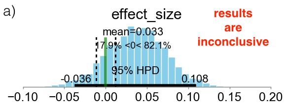
Below I am presenting three different scenarios. The cyan bars represent the distributions of the effect size defined in eq. (\ref{eq:effect_size}). The green vertical line represents the value ES=0, while the two vertical black broken lines define the ROPE as the locations where ES = $\pm 0.1$. In case (a), the 95% HPD is both inside and outside the ROPE and the experiment is considered inconclusive. In case (b), the 95% HPD is completely outside of the ROPE, on the right hand side of the green line. This means that the experiment is conclusive and group B is declared as the winner. In case (c), the 95% HPD is completely inside the ROPE and the experiment is also conclusive. In this case the “null value” is accepted and groups A and B are considered to be, effectively, as equivalent.
3.2 Option 2: Expected Loss Method
An alternative to the ROPE method is to calculate the Expected Loss that we would incur if we were to take the wrong decision. In other words, given the data observed in our experiment, what would be the cost associated in mistakenly declaring variant A (or variant B) as the winner? If this value is smaller than a certain “threshold of caring”, then we can declare variant A (or variant B) to be the winner. After all, if we were wrong the resulting loss would be so low that we would not… care. This method has been proposed by C. Stucchio [3].
The expected loss (due to making the wrong decision) is defined in the following way,
$$\begin{equation} \mathbb{E}(\mathcal{L}) = \min[\mathbb{E}(\mathcal{L}_A), \mathbb{E}(\mathcal{L}_B)] \label{eq:loss} \end{equation}$$
where $\mathbb{E}(\mathcal{L}_A)$ and $\mathbb{E}(\mathcal{L}_B)$ represent the expected losses associated with choosing “A” or “B” as the winners. These quantities are defined as
$$\begin{equation} \mathbb{E}(\mathcal{L}_A) = \int_0^1 \int_0^1\max(\mu_A - \mu_B,0)\,\mathbb{P}_A(\mu_A|\textbf{d}_A)\mathbb{P}_B(\mu_B|\textbf{d}_B)\,\textrm{d}\mu_A\textrm{d}\mu_B \label{eq:loss1} \end{equation}$$
and
$$\begin{equation} \mathbb{E}(\mathcal{L}_B) = \int_0^1 \int_0^1 \max(\mu_B - \mu_A,0)\,\mathbb{P}_A(\mu_A|\textbf{d}_A)\mathbb{P}_B(\mu_B|\textbf{d}_B)\,\textrm{d}\mu_A\textrm{d}\mu_B \label{eq:loss2} \end{equation}$$
In the expressions above, we have used the fact that the joint posterior $\mathbb{P}(\mu_A,\mu_B|\textbf{d}) = \mathbb{P}_A(\mu_A|\textbf{d}_A)\mathbb{P}_B(\mu_B|\textbf{d}_B)$, because the $\mu_A$ and $\mu_B$ distributions are independent. Also, note that the expected loss is always a positive number.
And here is our decision rule: if the expected loss, eq. (\ref{eq:loss}), is lower than our “threshold of caring”, we declare the experiment conclusive and we pick the variant with the smallest expected loss. If both expected losses, eqs. (\ref{eq:loss1}) and (\ref{eq:loss2}), are smaller than the threshold of caring, we declare the experiment conclusive and the two variations to be effectively equivalent.
One way to gain some more intuition on eqs. (\ref{eq:loss}), (\ref{eq:loss1}) and (\ref{eq:loss2}) is to reformulate the integrals in eqs. (\ref{eq:loss1}) and (\ref{eq:loss2}) in terms of the distribution of the lift, $\Delta \mu=\mu_B - \mu_A$. This allows us to transform those two-dimensional integrals into one-dimensional integrals over $\Delta \mu$.
In order to do so, we need to understand what is the distribution of the difference, $\mu_B - \mu_A$, given that we know only the distributions for $\mu_A$ and $\mu_B$. Luckily, there are plenty of references on the distribution of the sum of two random variables, stating that for independent random variables X and Y, with distributions $f_X(X)$ and $f_Y(Y)$, the distribution of the sum Z = X + Y equals the convolution of $f_X(X)$ and $f_Y(Y)$. Similarly, the distribution of the difference Z = X - Y equals the convolution of $f_X(X)$ and $f_Y(-Y)$.
Applying these concepts to our case, we can substitute $f_X(X)$ and $f_Y(Y)$ with $\mathbb{P}_A(\mu_A|\textbf{d}_A)$ and $\mathbb{P}_B(\mu_B|\textbf{d}_B)$, i.e. with the posterior distributions of the mean values $\mu_A$ and $\mu_B$. Then, the distribution of the difference $\Delta \mu = \mu_B - \mu_A$ looks like
$$\begin{equation} \mathbb{P}(\Delta\mu|\textbf{d}) = \int_0^1 \mathbb{P}_B(\mu_B|\textbf{d}_B)\mathbb{P}_A(\mu_B-\Delta\mu|\textbf{d}_A)\textrm{d}\mu_A\ \ , \end{equation}$$
which indeed represents the convolution of the distributions $\mu_A$ and $\mu_B$.
As mentioned above, we can use this to reduce the form for the expected loss $\mathbb{E}(\mathcal{L}_A)$ from a multi-dimensional integral to a one-dimensional integral over the posterior of the lift $\Delta\mu$,
$$\begin{equation} \mathbb{E}(\mathcal{L}_A) = \int_0^1 \int_0^1 \max(\mu_A - \mu_B,0)\,\mathbb{P}_A(\mu_A|\textbf{d}_A)\mathbb{P}_B(\mu_B|\textbf{d}_B)\,\textrm{d}\mu_A\textrm{d}\mu_B = \\ \int_0^1 \int_0^1 \max(-\Delta\mu,0)\,\mathbb{P}_B(\mu_B|\textbf{d}_B)\mathbb{P}_A(\mu_B-\Delta\mu|\textbf{d}_A)\textrm{d}\mu_A\textrm{d}\Delta\mu = \int_0^1 \max(-\Delta\mu,0)\,\mathbb{P}(\Delta\mu|\textbf{d})\textrm{d}\Delta\mu \label{eq:L1} \end{equation}$$
where the second equality comes from the substitution $\mu_A \rightarrow \mu_B - \Delta\mu$.
Similarly, for $\mathbb{E}(\mathcal{L}_B)$,
$$\begin{equation} \mathbb{E}(\mathcal{L}_B) = \int_0^1 \max(\Delta\mu,0)\,\mathbb{P}(\Delta\mu|\textbf{d})\textrm{d}\Delta\mu\ . \end{equation} \label{eq:L2}$$
As promised, we have obtained our one-dimensional integrals, eqs. (\ref{eq:L1}) and (\ref{eq:L2})! We can now plot the integrands in a simple Cartesian x-y axis. I hope this will help, as it has helped me understanding these concepts more deeply.
The expressions (\ref{eq:L1}) and (\ref{eq:L2}) tell us that the expected losses $\mathbb{E}(\mathcal{L}_A)$ and $\mathbb{E}(\mathcal{L}_B)$ are nothing more than the expected values of $\max(-\Delta\mu,0)$ and $\max(\Delta\mu,0)$ under the posterior distribution of the lift $\Delta\mu$.
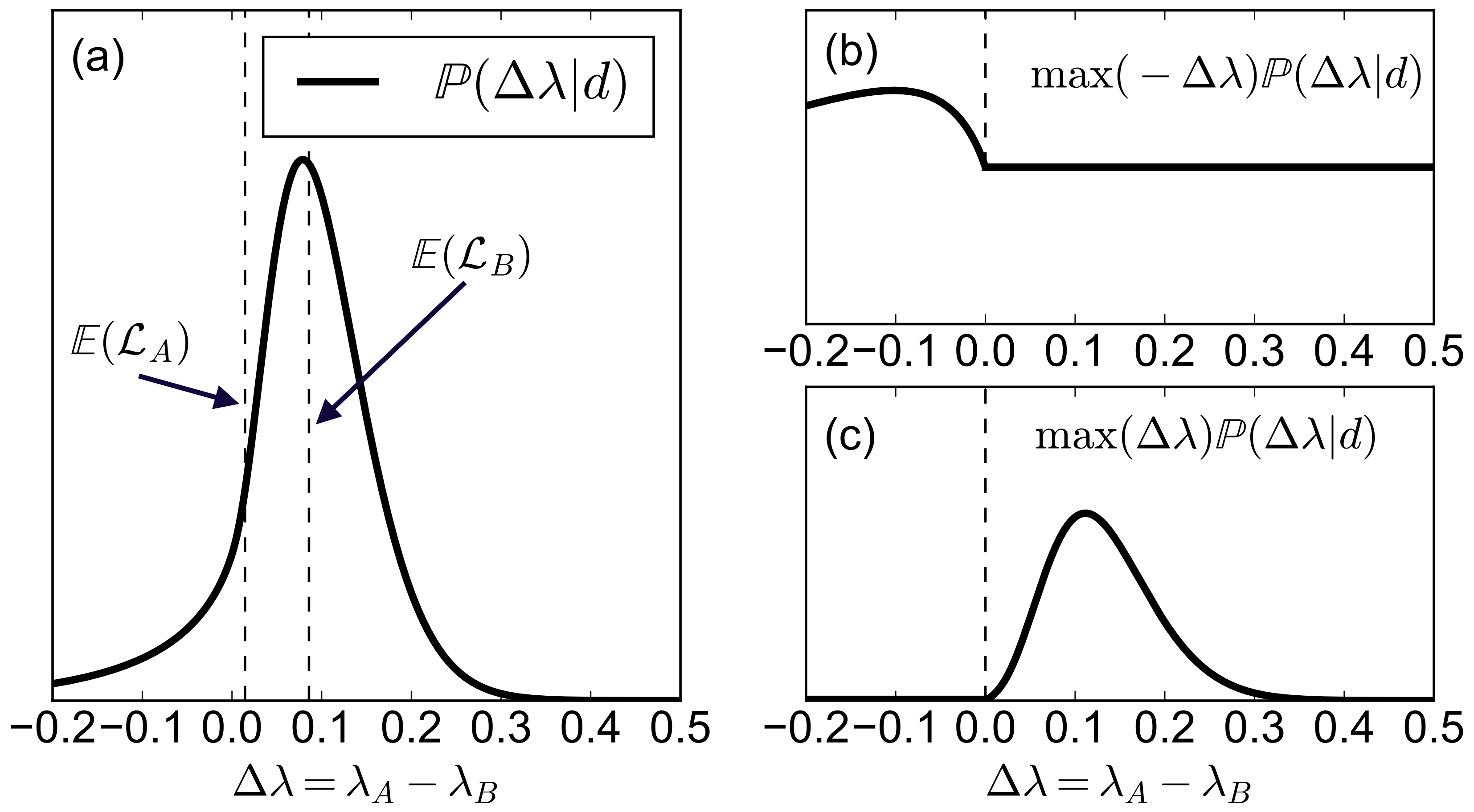
The figure below shows an example of a particular, arbitrary shape of $\mathbb{P}(\Delta\mu|d)$. Panel (a) shows the function $\mathbb{P}(\Delta\mu|d)$, together with the final values of the expected losses (broken lines). The integrands of eqs. (\ref{eq:L1}) and (\ref{eq:L2}) are displayed in the panels (b) and (c). The broken lines in (a) represent the values of $\mathbb{E}(\mathcal{L}_A)$ and $\mathbb{E}(\mathcal{L}_B)$.
3.3 Summary
We have seen how the ROPE and Expected Loss methods can be used as decision rules for our A/B experiments. Here I want to summarize how these methods should be applied.
ROPE Method
Expected Loss Method
At this point we have all the ingredients that are needed to understand and analyze an A/B experiment through the package aByes.
4. End-to-end Case Study
Let’s apply what we have learnt to a “real” scenario. More examples can be found in the aByes package, under the aByes/examples folder.
After having downloaded and installed the package, we import aByes using the command1
import abyes as ab
Next, we generate some random data. For this example, we are going to assume that the B variant does better than the A variant by picking values from a Bernoulli distribution with mean values of 0.5 and 0.4, respectively:
1 | data = [np.random.binomial(1, 0.4, size=10000), np.random.binomial(1, 0.5, size=10000)] |
The first element of this list is represented by a numpy array of size 10000, each element being a sample drawn by a Bernoulli distribution with probability of success of 0.4. Similarly, the second element is another numpy array of size 10000, but this time the probability of success is 0.5.
The data list represents our experimental data for the A and B buckets. Now let’s see how we can apply the different methods previously discussed to do a Bayesian analysis of these experimental results.
4.1 Analytic solution. Lift as decision variable, ROPE as decision rule.
In this scenario, we decide to analyze the experiment by applying the analytic method, with a decision variable based on the lift ($=\mu_B-\mu_A$) and a decision rule based on the ROPE. We choose the ROPE to be between -0.01 and 0.01 and use the 95% HPD region. This means that if there is more than a 95% chance that the absolute difference in conversion rate between the two variants is less than 1%, we declare the two variants to be effectively the same.
Here is how we can apply our Bayesian analysis to this case, using aByes,
1 | exp = ab.AbExp(method='analytic', decision_var = 'lift', rule='rope', rope=(-0.01,0.01), alpha=0.95, plot=True) |
Since we have used the flag plot=True, we will see the results in this plot:
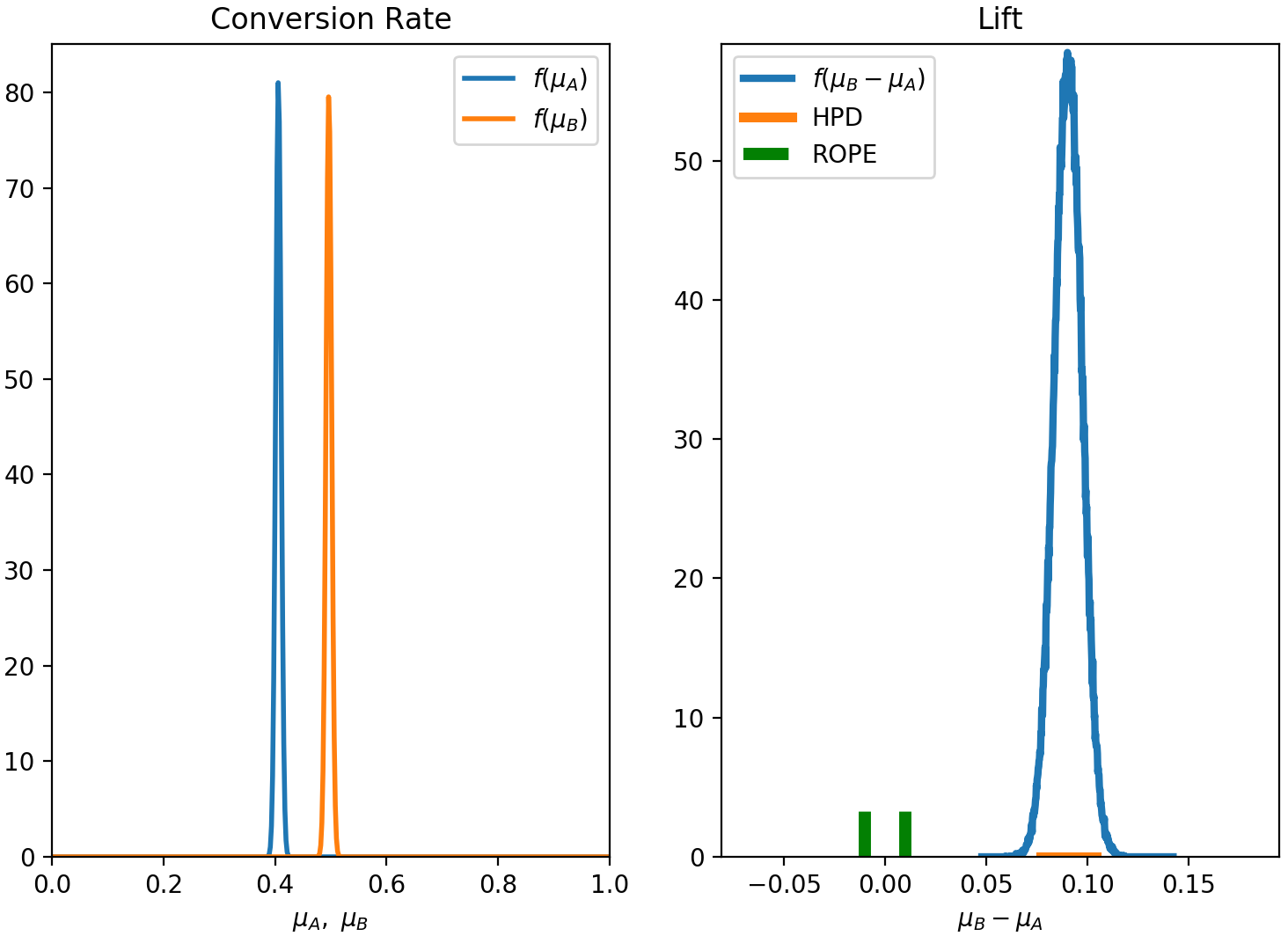
And here is the outcome of the experiment:
1 | *** abyes *** |
4.2 Analytic solution. Lift as decision variable, Expected Loss as decision rule.
This time we decide to use the Expected Loss as our decision rule and we set the threshold of caring to be 0.01 (this is also the default value),
1 | exp = ab.AbExp(method='analytic', decision_var = 'lift', rule='loss', toc=0.01, plot=True) |
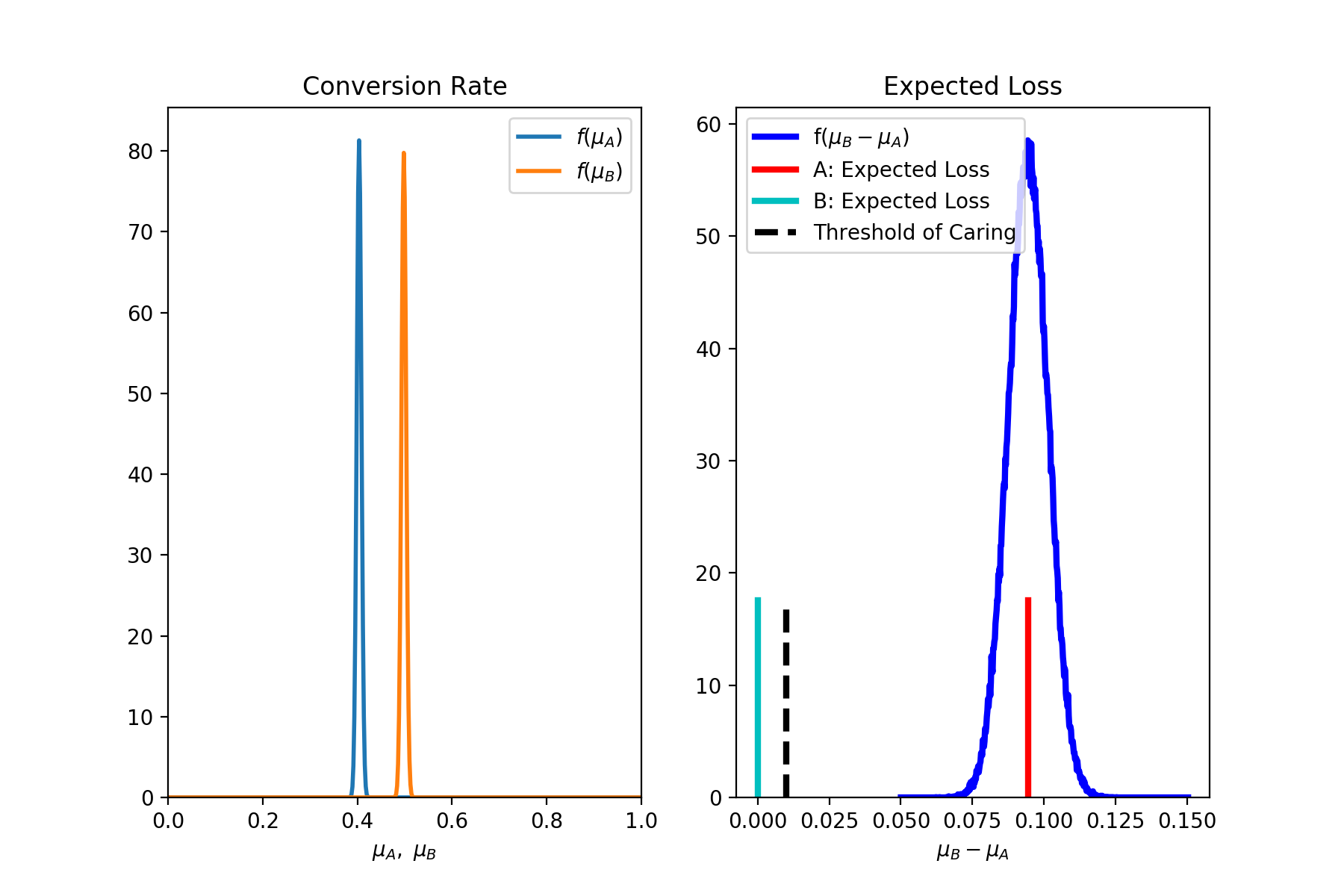
1 | *** abyes *** |
4.3 Numerical solution. Effect size as decision variable, ROPE as decision rule.
This time we use the numerical (MCMC) solution for our inference (you will need to have pyMC3 installed in your environment) and decide to use the effect size as our decision variable. In terms of decision rule, we again use the ROPE and set $\alpha=0.95$.
1 | exp = ab.AbExp(method='mcmc', decision_var = 'es', rule='rope', alpha=0.95, plot=True) |
I feel like it is always useful to plot the posterior distributions,
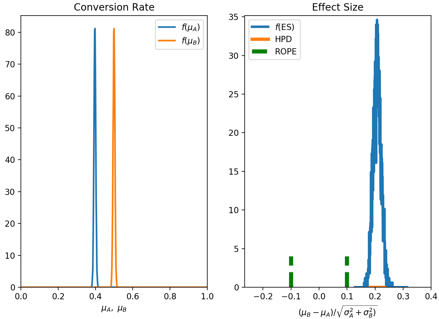
The outcome is the same as before: the B variant is the winner,
1 | *** abyes *** |
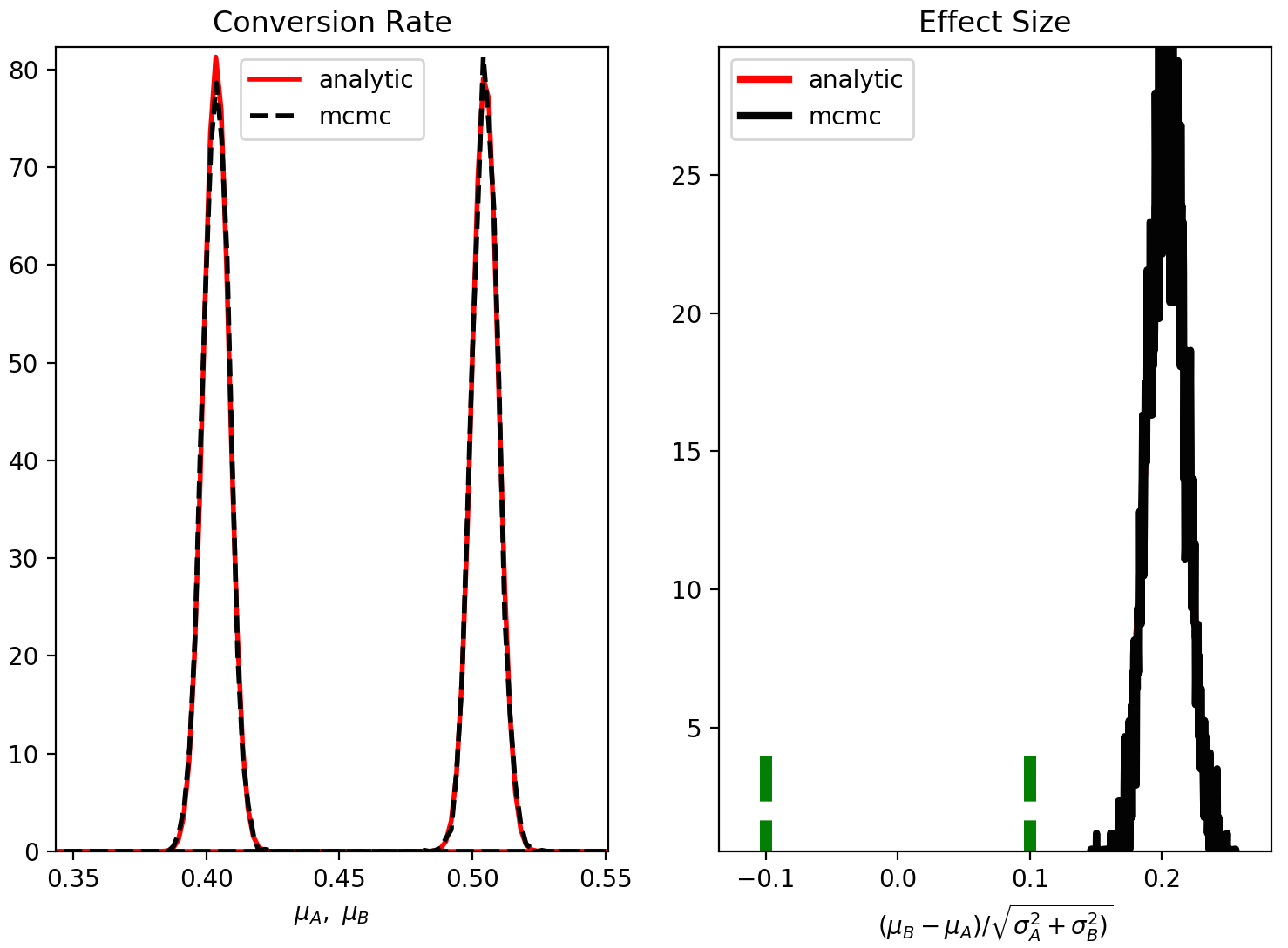
4.4 Bonus test. Compare analytic vs. numerical solution.
I have decided to add an extra option in aByes, which compares the analytic vs. numerical solutions. For standard conditions, the two solutions should actually be “identical”. This is an extra benchmark on the correctness of the code.
To see that the two methods agree to a very high degree, we can just type
1 | exp = ab.AbExp(method='compare', decision_var = 'es', plot=True) |
The resulting plot will show that, indeed, the posterior distributions from the analytic and MCMC solutions agree very well,
5. Summary and Conclusion
In this lengthy blog post, I have presented a detailed overview of Bayesian A/B Testing. From the first step of gathering the data to deciding whether to follow an analytic or numerical approach, to choosing the decision rule.
In the previous section, we have also seen some practical examples that make use of the Python package aByes.
Here are my suggestions for using aByes for conversion rate experiments:
- Use the analytic solution. There is no point in using the numerical solution at this stage of the aByes project, as it will give “identical” results to the analytic solution. Feel free to use the numerical solution if you are curious about MCMC methods. If you want to use a prior that is not well fitted by a Beta distribution, then you should definitely switch to the numerical solution (in this case you should also make some small changes the code to accommodate the distribution of your choice).
- In terms of choosing the decision variable, “lift” (difference in the mean conversion rates of the A and B variants) is the most easy to understand - so I would start from that. I believe “effect size” would be particularly useful for the analysis of revenue (rather than conversion rates), where the distributions can be skewed and it may be important to add information on the actual spread of the data away from the mean value.
- In choosing a decision rule, I don’t have a strong preference in favour of the ROPE or of the Expected Loss. At the moment I am fairly agnostic about it, with a slight preference towards the ROPE method as it seems to me to be more robust with respect to skewed distributions.
Thanks for reading this post. And remember to keep using your t-tests and chi-square tests when needed! :)
References
[1] A. D. I. Kramera, J. E. Guilloryb, and J. T. Hancock, Experimental evidence of massive-scale emotional contagion through social networks, PNAS, 111, 8788 (2013).
[2] J. K. Kruschke, Bayesian Estimation Supersedes the t Test, Journal of Experimental Psychology: General, 142, 573 (2013).
[3] C. Stucchio, Bayesian A/B Testing at VWO (2015).
[4] D. Hitchcock, Lecture notes available for the course STAT J535, Introduction to Bayesian Data Analysis, South Carolina University.
⁂