Since I have been really struggling to find an explanation of the backpropagation algorithm that I genuinely liked, I have decided to write this blogpost on the backpropagation algorithm for word2vec. My objective is to explain the essence of the backpropagation algorithm using a simple - yet nontrivial - neural network. Besides, word2vec has become so popular in the NLP community that it is quite useful to focus on it.

This blogpost is accompanied by another, more practical blogpost that you are <a href=/2018/01/07/backprop-word2vec-python/>invited to read. While this blogpost is going to be more theoretical (although there will be some examples), the other blogpost is focused on a Python implementation of everything discussed here.

Alright then, let’s start from what you need in order to really understand backpropagation. Aside from some basic concepts in machine learning (like knowing what is a loss function and the gradient descent algorithm), from a mathematical standpoint there are two main ingredients that you will need:

• some linear algebra (in particular, matrix multiplication)
• the chain rule for multivariate functions

If you know these concepts, what follows should be fairly easy. If you don’t master them yet, you should still be able to understand the reasoning behind the backpropagation algorithm. You may also want to <a href=/2018/01/07/backprop-word2vec-python/>skip directly to the Python implementation and come back to this blogpost when needed.

First of all, I would like to start with defining what the backpropagation algorithm really is. If this definition will not make much sense at the beginning, it should make much more sense later on.

1. What is the backpropagation algorithm?

Given a neural network, the parameters that the algorithm needs to learn in order to minimize the loss function are the weights of the network (N.B. I use the term weights in a loose sense, I also mean the bias terms). These are the only variables of the model, that are tweaked at every iteration until we arrive close to the minimum of the loss function.

In this context, backpropagation is an efficient algorithm that is used to find the optimal weights of a neural network: those that minimize the loss function. The standard way of finding these values is by applying the gradient descent algorithm, which implies finding out the derivatives of the loss function with respect to the weights.

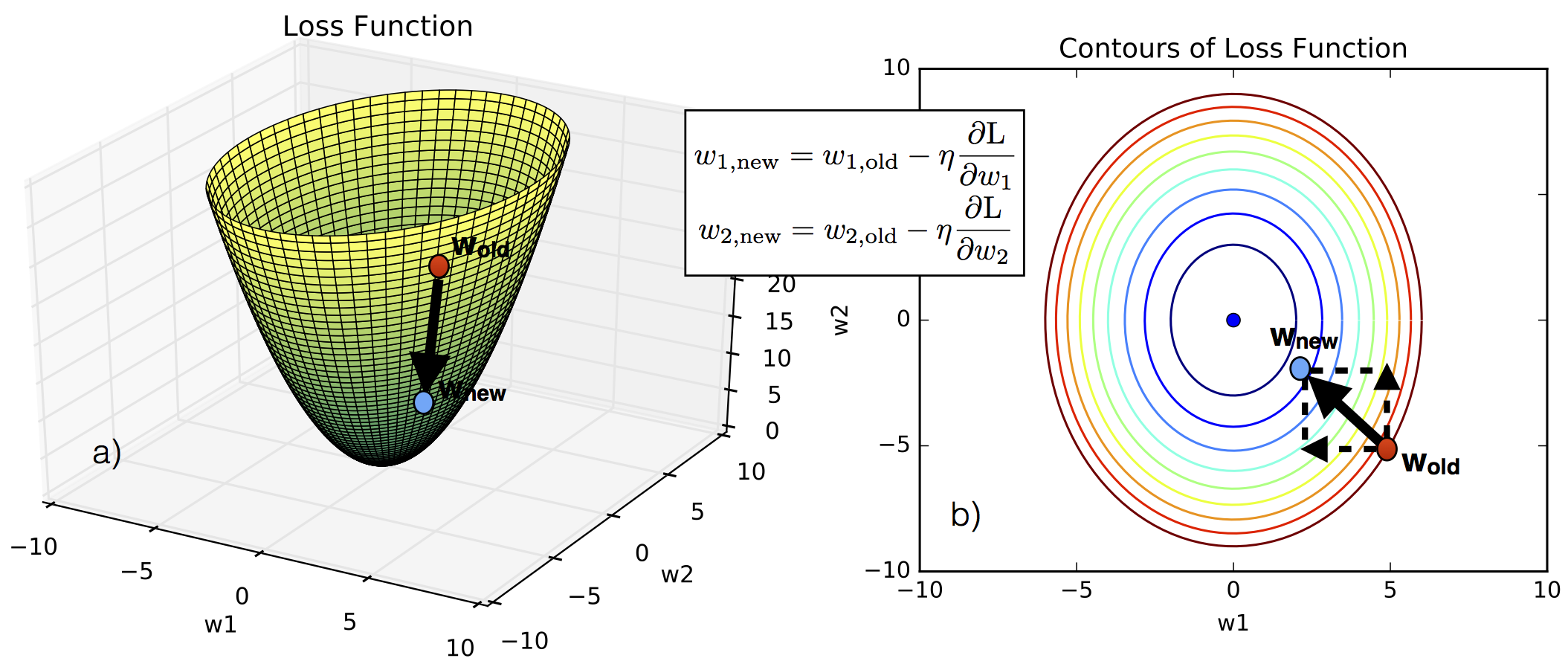
For trivial problems, those in which there are only two variables, it is easy to visualize how gradient descent works. If you look at the figure above, you will see in panel (a) a three-dimensional plot of the loss function as a function of the weights $w_1$ and $w_2$. At the beginning, we don’t know what their optimal values are, i.e., we don’t know which values of $w_1$ and $w_2$ minimize the loss function. Let’s say that we start from the red point. If we know how the loss function varies as we vary the value of the weights, i.e., if we know the derivatives $\partial\mathcal{L}/\partial w_1$ and $\partial\mathcal{L}/\partial w_2$, then we can move from the red point to a point closer to the minimum of the loss function, which is represented by a blue point in the figure. How far we move from the starting point is dictated by a parameter $\eta$ that is usually called learning parameter.

A big part of the backpropagation algorithm requires evaluating the derivatives of the loss function with respect to the weights. It is particularly instructive to see this for shallow neural networks, which is the case of word2vec.

2. Word2Vec

The objective of word2vec is to find word embeddings, given a text corpus. In other words, this is a technique for finding low-dimensional representations of words. As a consequence, when we talk about word2vec we are typically talking about Natural Language Processing (NLP) applications.

For example, a word2vec model trained with a 3-dimensional hidden layer will result in 3-dimensional word embeddings. It means that, say, the word “apartment” will be represented by a three-dimensional vector of real numbers that will be close (think of it in terms of Euclidean distance) to a similar word such as “house”. Put another way, word2vec is a technique for mapping words to numbers. Amazing eh?

There are two main models that are used within the context of word2vec: the Continuous Bag-of-Words (CBOW) and the Skip-gram model. We will be looking first at the simplest model, which is the Continuous Bag of Word (CBOW) model with a one-word window. We will then move to the multi-word window case and finally introduce the Skipgram model.

As we move along, I will present a few small examples with a text composed of only a few words. However, keep in mind that word2vec is typically trained with billions of words.

3. Continuous Bag Of Words (CBOW) single-word model in word2vec

In the CBOW model the objective is to find a target word $\hat{y}$, given a context of words (what this means will be clear soon). In the simplest case in which the word’s context is only represented by a single word, the neural network for the CBOW model looks like in the figure below,

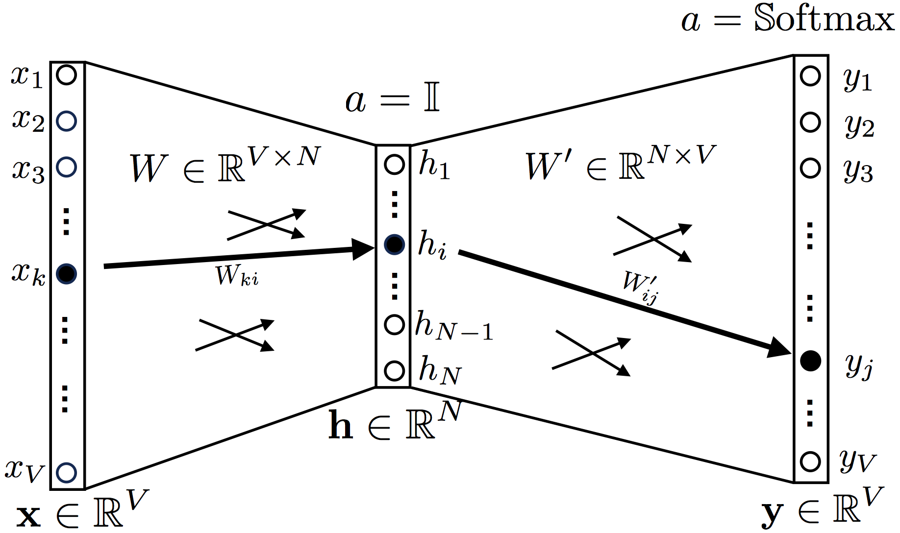
As you can see, there is one input layer, one hidden layer and finally an output layer. The activation function for the hidden layer is the identity $a=\mathbb{1}$ (usually, although improperly, called linear activation function). The activation function for the output is a softmax, $a=\mathbb{S}\textrm{oftmax}$.

The input layer is represented by a one-hot encoded vector $\textbf{x}$ of dimension V, where V is the size of the vocabulary. The hidden layer is defined by a vector of dimension N. Finally, the output layer is a vector of dimension V.

Now, let’s talk about weights: the weights between the input and the hidden layer are represented by a matrix $W$, of dimension $V\times N$. Similarly, the weigths between the hidden and the output layer are represented by a matrix $W’$, of dimension $N\times V$. For example, as in the figure, the relationship between an element $x_k$ of the input layer and an element $h_i$ of the hidden layer is represented by the weight $W_{ki}$. The connection between this node $h_i$ and an element $y_j$ of the output layer is represented by an element $W'_{ij}$.

The output vector $\textbf{y}$ will need to be compared against the expected targets $\hat{\textbf{y}}$. The closest is $\textbf{y}$ to $\hat{\textbf{y}}$, the better is the performance of the neural network (and the lower is the loss function).

If some of what you read so far sounds confusing, that’s because it always is! Have a look at the example below, it might clear things up!

Example

Suppose we want to train word2vec with the following text corpus:
$$\textrm{“I like playing football”}$$ We decide to train a simple CBOW model with one context word, just as in the Figure 2 above.

Given the text we have, our vocabulary will only be made of 4 words (hence, $V=4$). Also, we decide to only have two nodes in our hidden layer (hence, N=2). Our neural network will look like this:

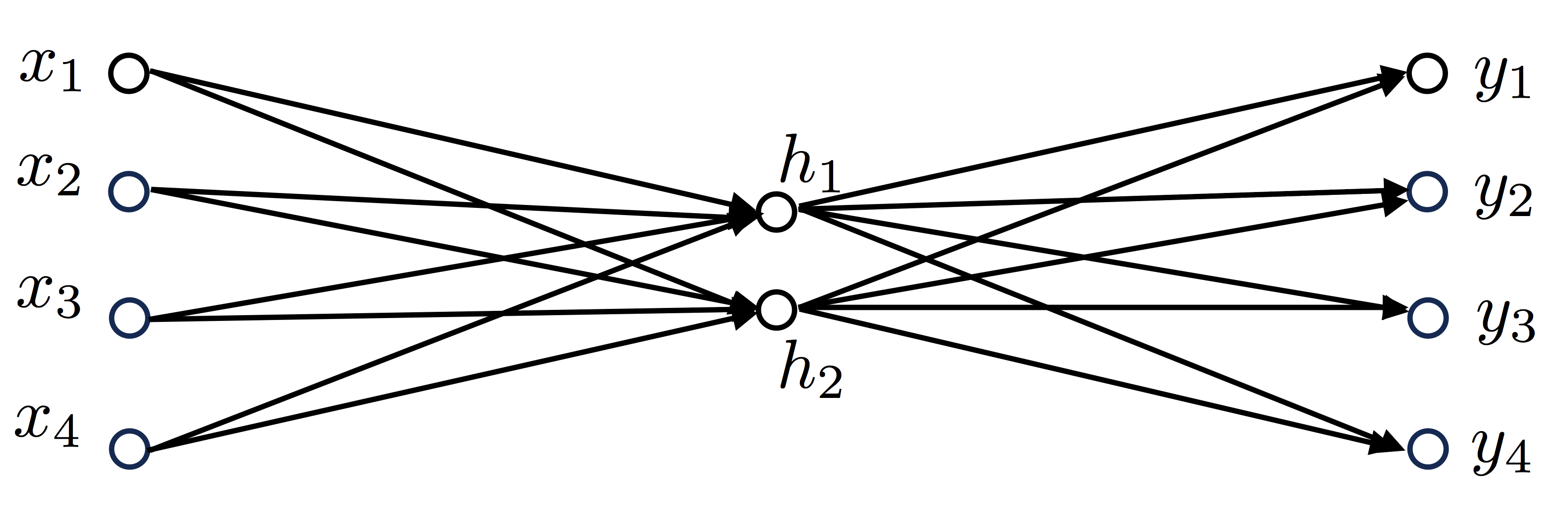
With the vocabulary being (in order of appearance):
$$\textrm{Vocabulary}=[\textrm{“I”}, \textrm{“like”}, \textrm{“playing”}, \textrm{“football”}]$$
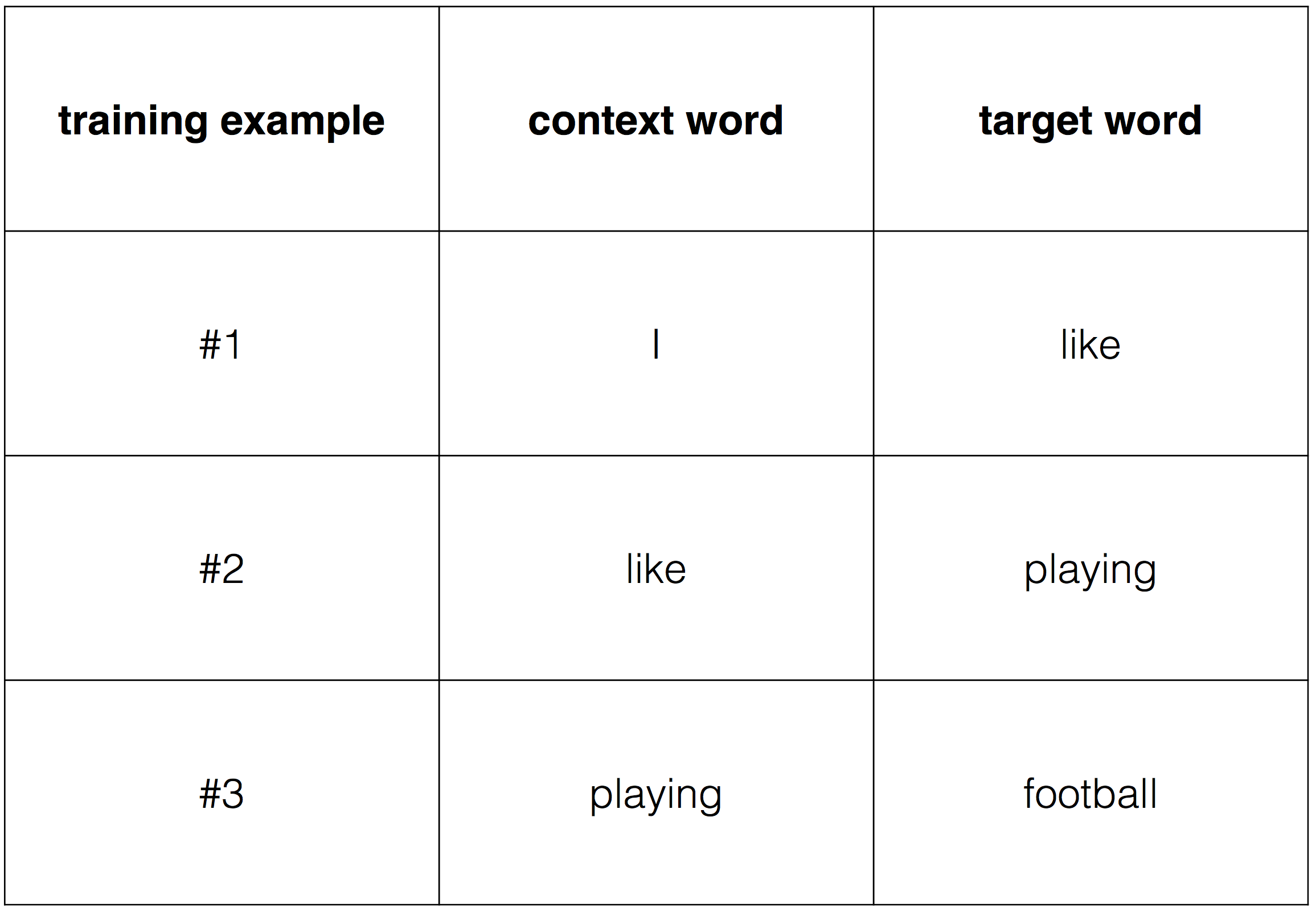
Next, we define as “target word” the word that follows a given word in the text (which becomes our “context word”). We can now construct our training examples, scanning the text with a window composed of a context word + a target word, like so:

For example, the target word for the context word “like” will be the word “playing”. Here is how our training data now looks like:

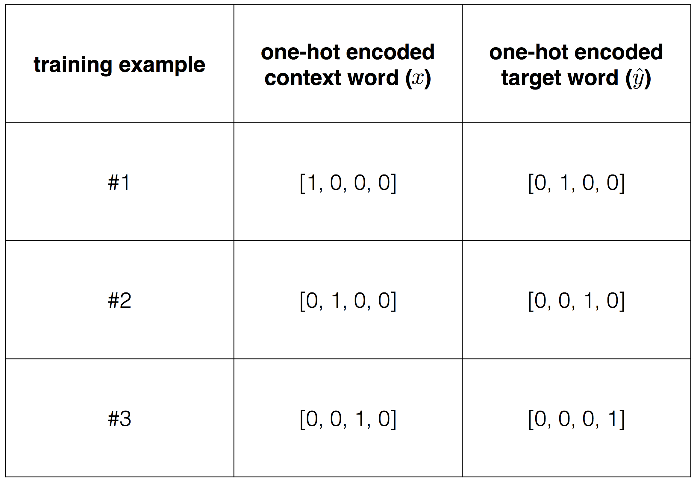
In order to feed this into an algorithm, we need to transform these data into numbers. In order to do so we use a one-hot encoding. For example the word “I”, which appears first in the vocabulary, will be encoded as the vector $[1, 0, 0, 0]$. The word “like”, which appears second in the vocaculary, will be encoded as the vector $[0, 1, 0, 0]$. The same would be for the target words, so the overall set of context-target words will be encoded as in the following table,

At this point we want to train our model, finding the weights that minimize the loss function. This corresponds to finding the weights that, given a context vector, can predict with the highest accuracy what is the corresponding target word $\hat{y}$.

3.1 Loss function

Given the topology of the network in Figure 1, let’s write down how to find the values of the hidden layer and of the output layer, given the input data $\textbf{x}$:

$$\begin{eqnarray*} \textbf{h} = & W^T\textbf{x} \hspace{7.0cm} \\ \textbf{u}= & W'^T\textbf{h}=W'^TW^T\textbf{x} \hspace{4.6cm} \\ \textbf{y}= & \ \ \mathbb{S}\textrm{oftmax}(\textbf{u})= \mathbb{S}\textrm{oftmax}(W'^TW^T\textbf{x}) \hspace{2cm} \end{eqnarray*}$$

where, following [1], $\textbf{u}$ is the value of the output before applying the $\mathbb{S}\textrm{oftmax}$ function.

Now, let’s say that we are training the model against the target-context word pair ($w_t, w_c$). The target word represents the ideal prediction from our neural network model, given the context word $w_c$. It is represented by a one-hot encoded vector. Say that it has value 1 at the position $j^*$ (and the value 0 for any other position).

The loss function will need to evaluate the output layer at the position $j^*$, or $y_{j^*}$ (the ideal value being equal to 1). Since the values in the softmax can be interpreted as conditional probabilities of the target word, given the context word $w_c$, we write the loss function as

$$\begin{equation*} \mathcal{L} = -\log \mathbb{P}(w_t|w_c)=-\log y_{j^*}\ =-\log[\mathbb{S}\textrm{oftmax}(u_{j^*})]=-\log\left(\frac{\exp{u_{j^*}}}{\sum_i \exp{u_i}}\right), \end{equation*}$$

where it is standard to add the log function. From the previous expression we obtain
$$\begin{equation} \bbox[lightblue,5px,border:2px solid red]{ \mathcal{L} = -u_{j^*} + \log \sum_i \exp{(u_i)}. } \label{eq:loss} \end{equation}$$

The loss function (\ref{eq:loss}) is the quantity we want to minimize, given our training example, i.e., we want to maximize the probability that our model predicts the target word, given our context word.

Example

Let’s go back to our previous example of the sentence “I like playing football”. Suppose we are training the model against the first training data point: the context word is “I” and the target word is “like”. Ideally, the values of the weights should be such that when the input $\textbf{x}=(1, 0, 0, 0)$ - which corresponds to the word “I” - then the output will be close to $\hat{\textbf{y}}=(0, 1, 0, 0)$ - which corresponds to the word “like”.

As standard for word2vec and in many neural networks, we can initialize the weights $W$ and $W’$ with standard normal distribution. For the sake of it, let’s say that the initial state of $W$, which is a $4\times 2$ matrix, is

$$W = \begin{pmatrix} -1.38118728 & 0.54849373 \\ 0.39389902 & -1.1501331 \\ -1.16967628 & 0.36078022 \\ 0.06676289 & -0.14292845 \end{pmatrix}$$
and the initial state of $W’$, which is a $2\times 4$ matrix, is
$$W' = \begin{pmatrix} 1.39420129 & -0.89441757 & 0.99869667 & 0.44447037 \\ 0.69671796 & -0.23364341 & 0.21975196 & -0.0022673 \end{pmatrix}$$
For the first training data “I like”, with context word $\textbf{x}=(1,0,0,0)^T$ and target word $\hat{\textbf{y}}=(0,0,1,0)^T$, we have
$$\textbf{h} = W^T\textbf{x}= \begin{pmatrix} -1.38118728 \\ 0.54849373 \end{pmatrix}$$
Then we have
$$\textbf{u} = W'^T\textbf{h}= \begin{pmatrix} -1.54350765 \\ 1.10720623 \\ -1.25885456 \\ -0.61514042 \end{pmatrix}$$
and finally
$$\textbf{y} = \mathbb{S}\textrm{oftmax}(\textbf{u})= \begin{pmatrix} 0.05256567 \\ 0.7445479 \\ 0.06987559 \\ 0.13301083 \end{pmatrix}$$
At this first iteration, the loss function will be the negative logarithm of the second element of $\textbf{y}$, or:
$$\mathcal{L}=-\log\mathbb{P}(\textrm{“like”}|\textrm{“I”})=-\log y_3 = -\log(0.7445479)= 0.2949781.$$ We could also calculate it using eq. (\ref{eq:loss}) , like so:
$$\begin{eqnarray*} \mathcal{L}=-u_2+\log\sum_{i=1}^4 u_i=-1.10720623 + \log[\exp(-1.54350765)+\exp(1.10720623) \\ +\exp(-1.25885456)+\exp(-0.61514042)]=0.2949781. \end{eqnarray*}$$At this point, before going into the next training example (“like”, “playing”), we have to change the weights of the network using gradient descent. How to do this? The backpropagation algorithm is the answer!

3.2 The backpropagation algorithm for the CBOW model

Now that we have an expression for the loss function, eq. (\ref{eq:loss}), we want to find the values of $W$ and $W’$ that minimize it. In the machine learning lingo, we want our model to “learn” the weights.

As we have seen in Section 1, in the neural networks world this optimization problem is usually tackled using gradient descent. Figure 1 shows how, in order to apply this method and update the weigth matrices $W$ and $W’$, we need to find the derivatives $\partial \mathcal{L}/\partial{W}$ and $\partial \mathcal{L}/\partial{W’}$.

I believe the easiest way to understand how to do this is to simply write down the relationship between the loss function and $W$, $W’$. Looking again at eq. (\ref{eq:loss}), it is clear that the loss function depends on the weights $W$ and $W’$ through the variable $\textbf{u}=[u_1, u_2, \dots, u_V]$, or

$$\begin{equation*} \mathcal{L} = \mathcal{L}(\mathbf{u}(W,W'))=\mathcal{L}(u_1(W,W'), u_2(W,W'),\dots, u_V(W,W'))\ . \end{equation*}$$

The derivatives then simply follow from the chain rule for multivariate functions,

$$\begin{equation} \frac{\partial\mathcal{L}}{\partial W'_{ij}} = \sum_{k=1}^V\frac{\partial\mathcal{L}}{\partial u_k}\frac{\partial u_k}{\partial W'_{ij}} \label{eq:dLdWp} \end{equation}$$

and

$$\begin{equation} \frac{\partial\mathcal{L}}{\partial W_{ij}} = \sum_{k=1}^V\frac{\partial\mathcal{L}}{\partial u_k}\frac{\partial u_k}{\partial W_{ij}}\ . \label{eq:dLdW} \end{equation}$$

And that’s it, this is pretty much the backpropagation algorithm! At this point we just need to specify eqs. (\ref{eq:dLdWp}) and (\ref{eq:dLdW}) for our usecase.

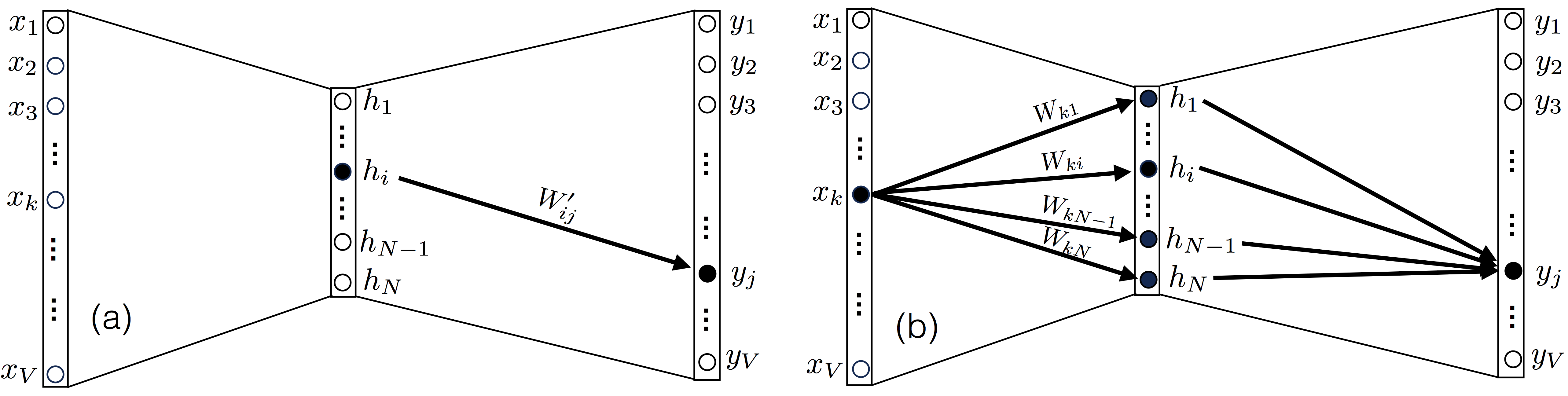
Let’s start from eq. (\ref{eq:dLdWp}). Note that the weight $W’_{ij}$, which is an element of the matrix $W’$ and connects a node $i$ of the hidden layer to a node $j$ of the output layer, only affects the output score $u_j$ (and also $y_j$), as seen in the panel (a) of the figure below,

Hence, among all the derivatives $\partial u_k/\partial W'_{ij}$, only the one where $k=j$ will be different from zero. In other words,
$$\begin{equation} \frac{\partial\mathcal{L}}{\partial W'_{ij}} = \frac{\partial\mathcal{L}}{\partial u_j}\frac{\partial u_j} {\partial W'_{ij}} \label{eq:derivative#1} \end{equation}$$

Let’s now calculate $\partial \mathcal{L}/\partial u_j$. We have
$$\begin{equation} \frac{\partial\mathcal{L}}{\partial u_j} = -\delta_{jj^*} + y_j := e_j \label{eq:term#1} \end{equation}$$
where $\delta_{jj^*}$ is a Kronecker delta: it is equal to 1 if $j=j^*$, otherwise it is equal to zero. In eq. (\ref{eq:term#1}) we have introduced the vector $\textbf{e} \in \mathbb{R}^V$, which is used to reduce the notational complexity. This vector represents the difference between the target (label) and the predicted output, i.e., it is the prediction error vector.
For the second term on the right hand side of eq. (\ref{eq:derivative#1}), we have
$$\begin{equation} \frac{\partial u_j}{\partial W'_{ij}} = \sum_{k=1}^V W_{ik}x_k \label{eq:term#2} \end{equation}$$
After inserting eqs. (\ref{eq:term#1}) and (\ref{eq:term#2}) into eq. (\ref{eq:derivative#1}), we obtain
$$\begin{equation} \bbox[white,5px,border:2px dotted red]{ \frac{\partial\mathcal{L}}{\partial W'_{ij}} = (-\delta_{jj^*} + y_j) \left(\sum_{k=1}^V W_{ki}x_k\right) } \label{eq:backprop1} \end{equation}$$

We can go through a similar exercise for the derivative $\partial\mathcal{L}/\partial W_{ij}$, however this time we note that after fixing the input $x_k$, the output $y_j$ at node $j$ depends on all the elements of the matrix $W$ that are connected to the input, as seen in Figure 3b. Therefore, this time we have to retain all the elements in the sum. Before going into the evaluation of $\partial u_k/\partial W_{ij}$, it is useful to write down the expression for the element $u_k$ of the vector $\textbf{u}$ as
$$\begin{equation*} u_k = \sum_{m=1}^N\sum_{l=1}^VW'_{mk}W_{lm}x_l\ . \end{equation*}$$
From this equation it is then easy to write down $\partial u_k/\partial W_{ij}$, since the only term that survives from the derivation will be the one in which $l=i$ and $m=j$, or
$$\begin{equation} \frac{\partial u_k}{\partial W_{ij}} = W'_{jk}x_i\ . \label{eq:term#3} \end{equation}$$
Finally, substituting eqs. (\ref{eq:term#1}) and (\ref{eq:term#3}) we get our well deserved result:
$$\begin{equation} \bbox[white,5px,border:2px dotted red]{ \frac{\partial \mathcal{L}}{\partial W_{ij}} = \sum_{k=1}^V (-\delta_{kk^*}+y_k)W'_{jk}x_i } \label{eq:backprop2} \end{equation}$$

Vectorization

We can simplify the notation of eqs. (\ref{eq:backprop1}) and (\ref{eq:backprop2}) by using a vector notation. Doing so, we obtain for eq. (\ref{eq:backprop1})
$$\begin{equation} \bbox[white,5px,border:2px dotted red]{ \frac{\partial\mathcal{L}}{\partial W'} = (W^T\textbf{x}) \otimes \textbf{e} } \end{equation}$$
where the symbol $\otimes$ denotes the outer product, that in Python can be obtained using the numpy.outer method.

For eq. (\ref{eq:backprop2}) we obtain
$$\begin{equation} \bbox[white,5px,border:2px dotted red]{ \frac{\partial \mathcal{L}}{\partial W} = \textbf{x}\otimes(W'\textbf{e}) } \end{equation}$$

3.3 Applying these results to gradient descent

Now that we have eqs. (\ref{eq:backprop1}) and (\ref{eq:backprop2}), we have all the ingredients needed to go through our first “learning” iteration, that consists in applying the gradient descent algorithm. This should have the effect of getting us a little closer to the minimum of the loss function. In order to apply gradient descent, after fixing a learning rate $\eta>0$ we can update the values of the weight vectors by using the equations
$$\begin{eqnarray} W_{\textrm{new}} & = W_{\textrm{old}} - \eta \frac{\partial \mathcal{L}}{\partial W} \nonumber \\ W'_{\textrm{new}} & = W'_{\textrm{old}} - \eta \frac{\partial \mathcal{L}}{\partial W'} \nonumber \\ \end{eqnarray}$$

3.4 Iterating the algorithm

What we have seen so far is only one small step of the entire optimization process. In particular, up to this point we have only trained the neural network with one single training example. In order to conclude the first pass, we have to go through all our training examples. Once we do this, we will have gone through a full epoch of optimization. At that point, most likely we will need to start again iterating through all our training data, until we reach a point in which we don’t observe big changes in the loss function. At that point, we can stop and declare that our neural network has been trained!

4. The backpropagation algorithm for the multi-word CBOW model

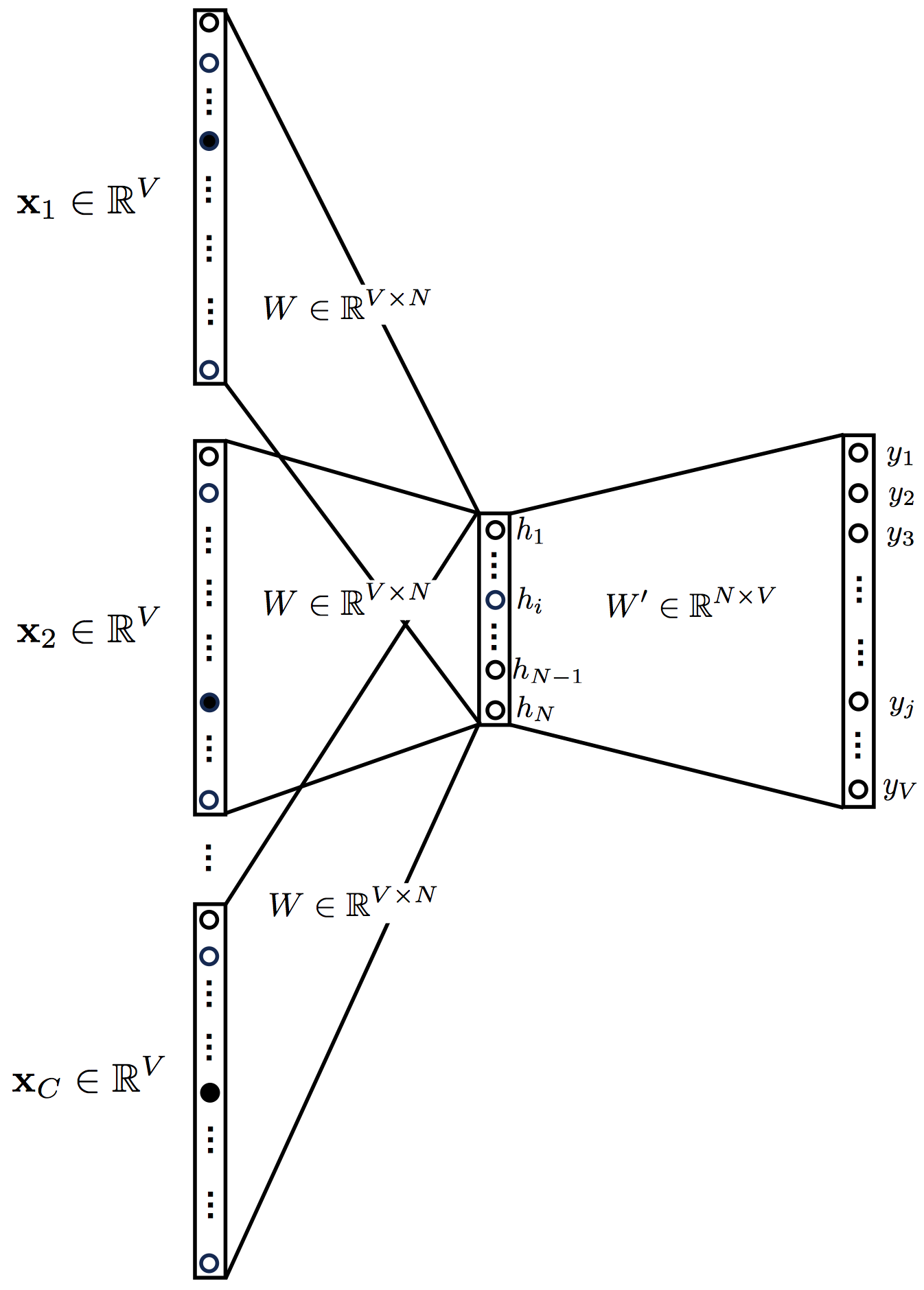
We know at this point how the backpropagation algorithm works for the one-word word2vec model. It is time to add an extra complexity by including more context words. Figure 4 shows how the neural network now looks. The input is given by a series of one-hot encoded context words, their number $C$ depending on our choice (how many context words we want to use). The hidden layer becomes an average of the values obtained from each context word.

The equations of the multi-word CBOW model are a generalization of the ones for the single-word CBOW model that we have already seen,
$$\begin{eqnarray} \textbf{h} = & \frac{1}{C} W^T \sum_{c=1}^C\textbf{x}^{(c)} = W^T\overline{\textbf{x}}\hspace{5.8cm} \nonumber \\ \textbf{u}= & W'^T\textbf{h}= \frac{1}{C}\sum_{c=1}^CW'^T W^T\textbf{x}^{(c)}=W'^T W^T\overline{\textbf{x}} \hspace{2.8cm} \nonumber \\ \textbf{y}= & \ \ \mathbb{S}\textrm{oftmax}(\textbf{u})= \mathbb{S}\textrm{oftmax}\left( W'^T W^T\overline{\textbf{x}}\right) \hspace{3.6cm} \nonumber \end{eqnarray}$$
Note that, for convenience, in the definitions above we have defined an “average” input vector $\overline{\textbf{x}}=\sum_{c=1}^C\textbf{x}^{(c)}/C$.

As before, in order to apply the backpropagation algorithm we need to write down the loss function and then look at its dependencies. The loss function looks just as before,
$$\begin{equation} \mathcal{L} = -\log\mathbb{P}(w_o|w_{c,1},w_{c,2},\dots,w_{c,C})=-u_{j^*} + \log \sum_i \exp{(u_i)}. \end{equation}$$
We write again the chain rules (identical to the previous ones),
$$\begin{equation} \frac{\partial\mathcal{L}}{\partial W'_{ij}} = \sum_{k=1}^V\frac{\partial\mathcal{L}}{\partial u_k}\frac{\partial u_k}{\partial W'_{ij}} \end{equation}$$
and
$$\begin{equation} \frac{\partial\mathcal{L}}{\partial W_{ij}} = \sum_{k=1}^V\frac{\partial\mathcal{L}}{\partial u_k}\frac{\partial u_k}{\partial W_{ij}}\ . \end{equation}$$
The derivatives of the loss function with respect to the weights are the same as for the single-word CBOW model, provided that we change the input vector with the average input vector. For completion, let’s derive these equations starting with the derivative with respect to $W’_{ij}$
$$\begin{equation} \frac{\partial\mathcal{L}}{\partial W'_{ij}} = \sum_{k=1}^V\frac{\partial\mathcal{L}}{\partial u_k}\frac{\partial u_k}{\partial W'_{ij}} = \frac{\partial\mathcal{L}}{\partial u_j}\frac{\partial u_j}{\partial W'_{ij}} = (-\delta_{jj^*} + y_j) \left(\sum_{k=1}^V W_{ki}\overline{x}_k\right) \end{equation}$$
and then writing the derivative with respect to $W_{ij}$,
$$\begin{equation} \frac{\partial\mathcal{L}}{\partial W_{ij}} = \sum_{k=1}^V\frac{\partial\mathcal{L}}{\partial u_k}\frac{\partial}{\partial W_{ij}}\left(\frac{1}{C}\sum_{m=1}^N\sum_{l=1}^V W'_{mk}\sum_{c=1}^C W_{lm}x_l^{(c)}\right)=\frac{1}{C}\sum_{k=1}^V\sum_{c=1}^C(-\delta_{kk^*} + y_k)W'_{jk}x_i^{(c)} . \end{equation}$$
Summarizing, for the multi-word CBOW model we have
$$\begin{equation} \bbox[white,5px,border:2px dotted red]{ \frac{\partial\mathcal{L}}{\partial W'_{ij}} = (-\delta_{jj^*} + y_j) \left(\sum_{k=1}^V W_{ki}\overline{x}_k\right) } \label{eq:backprop1_multi} \end{equation}$$
and
$$\begin{equation} \bbox[white,5px,border:2px dotted red]{ \frac{\partial\mathcal{L}}{\partial W_{ij}} = \sum_{k=1}^V(-\delta_{kk^*} + y_k)W'_{jk}\overline{x}_i . } \label{eq:backprop2_multi} \end{equation}$$

Vectorization

Once again, it is extremely useful to write eqs. (\ref{eq:backprop1_multi}) and (\ref{eq:backprop2_multi}) using vector notation. We start with eq. (\ref{eq:backprop1_multi})
$$\begin{equation} \bbox[white,5px,border:2px dotted red]{ \frac{\partial\mathcal{L}}{\partial W'} = (W^T\overline{\textbf{x}}) \otimes \textbf{e} } \end{equation}$$
where the symbol $\otimes$ denotes the outer product.

For eq. (\ref{eq:backprop2_multi}), we have
$$\begin{equation} \bbox[white,5px,border:2px dotted red]{ \frac{\partial \mathcal{L}}{\partial W} =\overline{\textbf{x}}\otimes(W'\textbf{e}) } \end{equation}$$

Note how these equations are identical to the ones for the single-word CBOW model, the only difference being that we have replaced a single input vector with an averaged one.

5. The backpropagation algorithm for the Skip-gram model

The Skip-gram model is essentially the inverse of the CBOW model. The input is a center word and the output predicts the context words, given the center word. The resulting neural network looks like in the figure below,

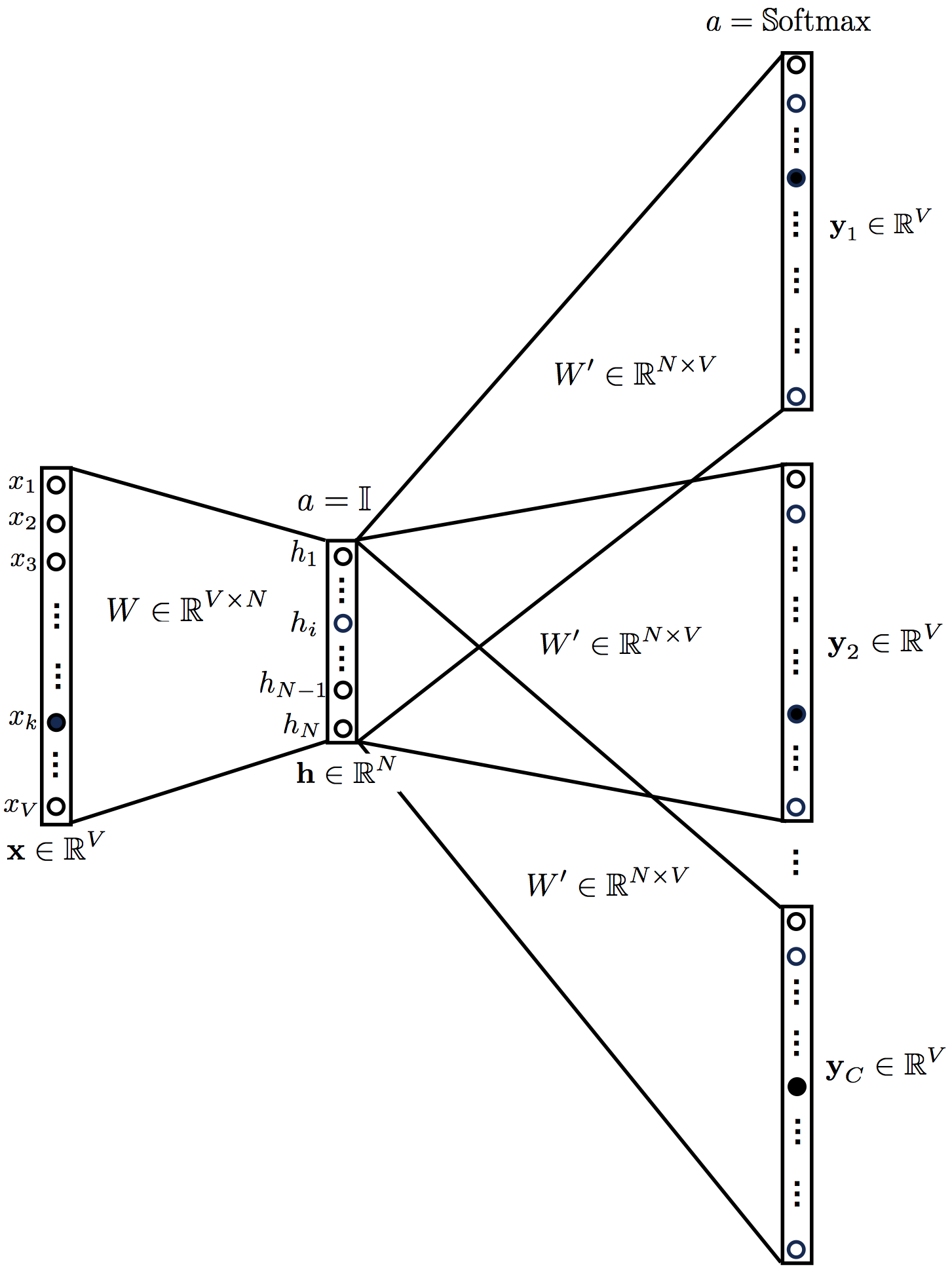
The equations of the Skip-gram model are the following,
$$\begin{eqnarray*} \textbf{h} = & W^T\textbf{x} \hspace{9.4cm} \\ \textbf{u}_c= & W'^T\textbf{h}=W'^TW^T\textbf{x} \hspace{4cm} c=1, \dots, C \hspace{0.7cm}\\ \textbf{y}_c = & \ \ \mathbb{S}\textrm{oftmax}(\textbf{u})= \mathbb{S}\textrm{oftmax}(W'^TW^T\textbf{x}) \hspace{2cm} c=1, \dots, C \end{eqnarray*}$$

Note that the output vectors (as well as the vectors $\textbf{u}_c$) are all identical, $\mathbf{y}_1=\mathbf{y}_2\dots= \mathbf{y}_C$. The loss function for the Skip-gram model looks like this:
$$\begin{eqnarray*} \mathcal{L} = -\log \mathbb{P}(w_{c,1}, w_{c,2}, \dots, w_{c,C}|w_o)=-\log \prod_{c=1}^C \mathbb{P}(w_{c,i}|w_o) \\ = -\log \prod_{c=1}^C \frac{\exp(u_{c,j^*})}{\sum_{j=1}^V \exp(u_{c,j})} =-\sum_{c=1}^C u_{c,j^*} + \sum_{c=1}^C \log \sum_{j=1}^V \exp(u_{c,j}) \end{eqnarray*}$$

For the Skip-gram model, the loss function depends on $C\times V$ variables via
$$\begin{equation*} \mathcal{L} = \mathcal{L}(\mathbf{u_1}(W,W'), \mathbf{u_2}(W,W'), \dots, \mathbf{u_C}(W,W'))=\mathcal{L}(u_{1,1}(W,W'), u_{1,2}(W,W'), \dots, u_{C,V}(W,W')) \end{equation*}$$

Therefore in this case the chain rule reads
$$\begin{equation*} \frac{\partial\mathcal{L}}{\partial W'_{ij}} = \sum_{k=1}^V\sum_{c=1}^C\frac{\partial\mathcal{L}}{\partial u_{c,k}}\frac{\partial u_{c,k}}{\partial W'_{ij}} \end{equation*}$$
and
$$\begin{equation*} \frac{\partial\mathcal{L}}{\partial W_{ij}} = \sum_{k=1}^V\sum_{c=1}^C\frac{\partial\mathcal{L}}{\partial u_{c,k}}\frac{\partial u_{c,k}}{\partial W_{ij}}\ . \end{equation*}$$
Let’s now calculate $\partial \mathcal{L}/\partial u_{c,j}$. We have
$$\begin{equation*} \frac{\partial\mathcal{L}}{\partial u_{c,j}} = -\delta_{jj_c^*} + y_{c,j} := e_{c,j} \end{equation*}$$

Similarly as for the CBOW model, we get
$$\begin{equation*} \frac{\partial\mathcal{L}}{\partial W'_{ij}} = \sum_{k=1}^V\sum_{c=1}^C\frac{\partial\mathcal{L}}{\partial u_{c,k}}\frac{\partial u_{c,k}}{\partial W'_{ij}} = \sum_{c=1}^C\frac{\partial\mathcal{L}}{\partial u_{c,j}}\frac{\partial u_{c,j}}{\partial W'_{ij}} = \sum_{c=1}^C(-\delta_{jj_c^*} + y_{c,j}) \left(\sum_{k=1}^V W_{ki}x_k\right) \end{equation*}$$
The derivative with respect to $W_{ij}$ is the most complicated one, but still feasible:
$$\begin{equation*} \frac{\partial\mathcal{L}}{\partial W_{ij}} = \sum_{k=1}^V\sum_{c=1}^C\frac{\partial\mathcal{L}}{\partial u_{c,k}}\frac{\partial}{\partial W_{ij}}\left(\sum_{m=1}^N\sum_{l=1}^V W'_{mk} W_{lm}x_l\right)=\sum_{k=1}^V\sum_{c=1}^C (-\delta_{kk_c^*} + y_{c,k})W'_{jk}x_i . \end{equation*}$$
Summarizing, for the Skip-Gram model we have
$$\begin{equation} \bbox[white,5px,border:2px dotted red]{ \frac{\partial\mathcal{L}}{\partial W'_{ij}} = \sum_{c=1}^C(-\delta_{jj_c^*} + y_{c,j}) \left(\sum_{k=1}^V W_{ki}x_k\right) } \label{eq:backprop1_skip} \end{equation}$$
and
$$\begin{equation} \bbox[white,5px,border:2px dotted red]{ \frac{\partial\mathcal{L}}{\partial W_{ij}} = \sum_{k=1}^V\sum_{c=1}^C (-\delta_{kk_c^*} + y_{c,k})W'_{jk}x_i . } \label{eq:backprop2_skip} \end{equation}$$

Vectorization

Here is the vectorized version of eq. (\ref{eq:backprop1_skip})
$$\begin{equation} \bbox[white,5px,border:2px dotted red]{ \frac{\partial\mathcal{L}}{\partial W'} = (W^T\textbf{x}) \otimes \sum_{c=1}^C\textbf{e}_c } \end{equation}$$
where the symbol $\otimes$ denotes the outer product.

For eq. (\ref{eq:backprop2_skip}), we get
$$\begin{equation} \bbox[white,5px,border:2px dotted red]{ \frac{\partial \mathcal{L}}{\partial W} = \textbf{x}\otimes\left(W'\sum_{c=1}^C\textbf{e}_c\right) } \end{equation}$$

6. What’s Next

We have seen in detail how the backpropagation algorithm works for the word2vec usecase. However, it turns out that the implementations we have seen are not computationally efficient for large text corpora. The original paper [2] introduced some “tricks” useful to overcome this difficulty (Hierarchical Softmax and Negative Sampling), but I am not going to cover them here. You can find a good explanation in [1].

Despite being computationally inefficient, the implementations discussed here contain everything that is needed in order to train word2vec neural networks. The next step would then be to implement these equations in your favourite programming language. If you like Python, I have already implemented these equations for you. I discuss about them in <a href=/2018/01/07/backprop-word2vec-python/>my next blogpost. Maybe I’ll see you there!

References

[1] X. Rong, word2vec Parameter Learning Explained, arXiv:1411.2738 (2014) .
[2] T. Mikolov, K. Chen, G. Corrado, J. Dean, Efficient Estimation of Word Representations in Vector Space, arXiv:1301.3781 (2013).

Today’s Mondrian random generator