In this blogpost, I will show you how to implement word2vec using the standard Python library, NumPy and two utility functions from Keras. A more complete codebase can be found under my Github webpage, with a project named word2veclite. This codebase also contains a set of unit tests that compare the solution described in this blogpost against the one obtained using Tensorflow.
Our starting point is the theoretical discussion on word2vec that I presented in my previous blogpost. In particular, the objective here is to implement the vectorized expressions presented in that blogpost, since they are compact and computationally efficient. We will be simply coding up a few of those equations.
1. Requirements
For this tutorial we will be using Python 3.6. The packages that we will need are NumPy (I am using version 1.13.3) and Keras (version 2.0.9). Here Keras is only used because of a few useful NLP tools (Tokenizer, sequence and np_utils). At the end of the blogpost I am also going to add a brief discussion on how to implement wordvec in Tensorflow (version 1.4.0), so you may want to import that as well.1
2
3
4
5import numpy as np
from keras.preprocessing.text import Tokenizer
from keras.preprocessing import sequence
from keras.utils import np_utils
import tensorflow as tf
2. From corpus to center and context words
The first step in our implementation is to transform a text corpus into numbers. Specifically, into one-hot encoded vectors. Recall that in word2vec we scan through a text corpus and for each training example we define a center word with its surrounding context words. Depending on the algorithm of choice (Continuous Bag-of-Words or Skip-gram), the center and context words may work as inputs and labels, respectively, or vice versa.
Typically the context words are defined as a symmetric window of predefined length, on both the left and right hand sides of the center word. For example, suppose our corpus consists of the sentence “I like playing football with my friends”. Also, let’s say that we define our window to be symmetric around the center word and of length two. Then, our one-hot encoded context and center words can be visualized as follows,
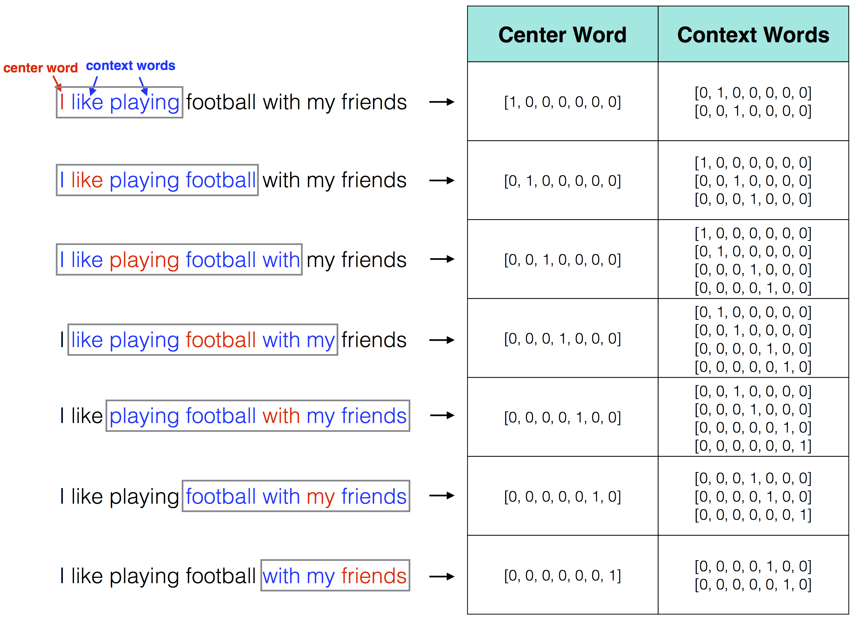
Note that at the boundaries the context words are not symmetric around the center words.
We are essentially interested in writing a few lines of code that accomplish this mapping, from text to one-hot-encoded vectors, as displayed in the figure above. In order to do so, first we need to tokenize the corpus text.1
2
3
4
5
6
7
8
9
10
11def tokenize(corpus):
"""Tokenize the corpus text.
:param corpus: list containing a string of text (example: ["I like playing football with my friends"])
:return corpus_tokenized: indexed list of words in the corpus, in the same order as the original corpus (the example above would return [[1, 2, 3, 4]])
:return V: size of vocabulary
"""
tokenizer = Tokenizer()
tokenizer.fit_on_texts(corpus)
corpus_tokenized = tokenizer.texts_to_sequences(corpus)
V = len(tokenizer.word_index)
return corpus_tokenized, V
The function above returns the corpus tokenized and the size $V$ of the vocabulary. The vocabulary is not sorted in alphabetical order (it is not necessary to do so) but it simply follows the order of appearance.
At this point we can proceed with the mapping from text to one-hot encoded context and center words using the function corpus2io which uses the auxiliary function to_categorical (copied from the Keras repository).1
2
3
4
5
6
7
8
9
10
11
12
13
14
15
16
17
18
19
20
21
22
23
24
25
26
27
28
29
30
31
32
33
34
35
36
37
38
39
40
41
42
43
44def to_categorical(y, num_classes=None):
"""Converts a class vector (integers) to binary class matrix.
E.g. for use with categorical_crossentropy.
# Arguments
y: class vector to be converted into a matrix
(integers from 0 to num_classes).
num_classes: total number of classes.
# Returns
A binary matrix representation of the input.
"""
y = np.array(y, dtype='int')
input_shape = y.shape
if input_shape and input_shape[-1] == 1 and len(input_shape) > 1:
input_shape = tuple(input_shape[:-1])
y = y.ravel()
if not num_classes:
num_classes = np.max(y) + 1
n = y.shape[0]
categorical = np.zeros((n, num_classes))
categorical[np.arange(n), y] = 1
output_shape = input_shape + (num_classes,)
categorical = np.reshape(categorical, output_shape)
return categorical
def corpus2io(corpus_tokenized, V, window_size):
"""Converts corpus text into context and center words
# Arguments
corpus_tokenized: corpus text
window_size: size of context window
# Returns
context and center words (arrays)
"""
for words in corpus_tokenized:
L = len(words)
for index, word in enumerate(words):
contexts = []
labels = []
s = index - window_size
e = index + window_size + 1
contexts.append([words[i]-1 for i in range(s, e) if 0 <= i < L and i != index])
labels.append(word-1)
x = np_utils.to_categorical(contexts, V)
y = np_utils.to_categorical(labels, V)
yield (x, y.ravel())
And that’s it! To show that the functions defined above do accomplish the required task, we can replicate the example presented in Fig. 1. First, we define the size of the window and the corpus text. Then, we tokenize the corpus and apply the corpus2io function defined above to find out the one-hot encoded arrays of context and center words:1
2
3
4
5window_size = 2
corpus = ["I like playing football with my friends"]
corpus_tokenized, V = tokenize(corpus)
for i, (x, y) in enumerate(corpus2io(corpus_tokenized, V, window_size)):
print(i, "\n center word =", y, "\n context words =\n",x)
Show output
1 | 0 |
4. Softmax function
One function that is particularly important in word2vec (and in any multi-classification problems) is the Softmax function. A simple implementation of this function is the following,
1 | def softmax(x): |
Given an array of real numbers (including negative ones), the softmax function essentially returns a probability distribution with sum of the entries equal to one.
Note that the implementation above is slightly more complex than the naïve implementation that would simply return np.exp(x) / np.sum(np.exp(x)). However, it has the advantage of being superior in terms of numerical stability.
Example
The following example
1 | data = [-1, -5, 1, 5, 3] |
will print the results:
1 | softmax(data) = [2.1439e-03 3.9267e-05 1.5842e-02 8.6492e-01 1.1705e-01] |
4. Python code for the Multi-Word CBOW model
Now that we can build training examples and labels from a text corpus, we are ready to implement our word2vec neural network. In this section we start with the Continuous Bag-of-Words model and then we will move to the Skip-gram model.
You should remember that in the CBOW model the input is represented by the context words and the labels (ground truth) by the center words. The full set of equations that we need to solve for the CBOW model are (see the section on the multi-word CBOW model in my previous blog post):
$$\begin{eqnarray} \textbf{h} = & W^T\overline{\textbf{x}}\hspace{2.8cm} \nonumber \\ \textbf{u} = & W'^T W^T\overline{\textbf{x}} \hspace{2cm} \nonumber \\ \textbf{y} = & \mathbb{S}\textrm{oftmax}\left( W'^T W^T\overline{\textbf{x}}\right) \hspace{0cm} \nonumber \\ \mathcal{L} = & -u_{j^*} + \log \sum_i \exp{(u_i)} \hspace{0cm} \nonumber \\ \frac{\partial\mathcal{L}}{\partial W'} = & (W^T\overline{\textbf{x}}) \otimes \textbf{e} \hspace{2.0cm} \nonumber\\ \frac{\partial \mathcal{L}}{\partial W} = & \overline{\textbf{x}}\otimes(W'\textbf{e}) \hspace{2.0cm} \nonumber \end{eqnarray}$$Then, we apply gradient descent to update the weights:
$$\begin{eqnarray}
W_{\textrm{new}} = W_{\textrm{old}} - \eta \frac{\partial \mathcal{L}}{\partial W} \nonumber \\
W'_{\textrm{new}} = W'_{\textrm{old}} - \eta \frac{\partial \mathcal{L}}{\partial W'} \nonumber \\
\end{eqnarray}$$
Seems complicated? Not really, each equation above can be coded up in a single line of Python code. In fact, right below is a function that solves all the equations for the CBOW model:1
2
3
4
5
6
7
8
9
10
11
12
13
14
15
16
17
18
19
20
21
22
23
24
25def cbow(context, label, W1, W2, loss):
"""
Implementation of Continuous-Bag-of-Words Word2Vec model
:param context: all the context words (these represent the inputs)
:param label: the center word (this represents the label)
:param W1: weights from the input to the hidden layer
:param W2: weights from the hidden to the output layer
:param loss: float that represents the current value of the loss function
:return: updated weights and loss
"""
x = np.mean(context, axis=0)
h = np.dot(W1.T, x)
u = np.dot(W2.T, h)
y_pred = softmax(u)
e = -label + y_pred
dW2 = np.outer(h, e)
dW1 = np.outer(x, np.dot(W2, e))
new_W1 = W1 - eta * dW1
new_W2 = W2 - eta * dW2
loss += -float(u[label == 1]) + np.log(np.sum(np.exp(u)))
return new_W1, new_W2, loss
It needs, as input, numpy arrays of context words and labels as well as the weights and the current value of the loss function. As output, it returns the updated values of the weights and loss.
Here is an example on how to use this function:1
2
3
4
5
6
7
8
9
10
11
12
13
14
15
16
17
18#user-defined parameters
corpus = ["I like playing football with my friends"] #our example text corpus
N = 2 #assume that the hidden layer has dimensionality = 2
window_size = 2 #symmetrical
eta = 0.1 #learning rate
corpus_tokenized, V = tokenize(corpus)
#initialize weights (with random values) and loss function
np.random.seed(100)
W1 = np.random.rand(V, N)
W2 = np.random.rand(N, V)
loss = 0.
for i, (context, label) in enumerate(corpus2io(corpus_tokenized, V, window_size)):
W1, W2, loss = cbow(context, label, W1, W2, loss)
print("Training example #{} \n-------------------- \n\n \t label = {}, \n \t context = {}".format(i, label, context))
print("\t W1 = {}\n\t W2 = {} \n\t loss = {}\n".format(W1, W2, loss))
Show output
1 | Training example #0 |
As a further note, the output shown above represents a single epoch, i.e., a single pass through the training examples. In order to train a full model it is necessary to iterate across several epochs. We will see this in section 7.
5. Python code for the Skip-Gram model
In the skip-gram model, the inputs are represented by center words and the labels by context words. The full set of equations that we need to solve are the following (see the section on the skip-gram model in my previous blog post):
$$\begin{eqnarray}
\textbf{h} = & W^T\textbf{x} \hspace{9.5cm} \nonumber \\
\textbf{u}_c= & W'^T\textbf{h}=W'^TW^T\textbf{x} \hspace{3cm} \hspace{2cm} c=1, \dots , C \nonumber \\
\textbf{y}_c = & \ \ \mathbb{S}\textrm{oftmax}(\textbf{u})= \mathbb{S}\textrm{oftmax}(W'^TW^T\textbf{x}) \hspace{2.3cm} c=1, \dots , C \nonumber \\
\mathcal{L} = & -\sum_{c=1}^C u_{c,j^*} + \sum_{c=1}^C \log \sum_{j=1}^V \exp(u_{c,j}) \hspace{5cm} \nonumber \\
\frac{\partial\mathcal{L}}{\partial W'} = & (W^T\textbf{x}) \otimes \sum_{c=1}^C\textbf{e}_c \hspace{7.7cm} \nonumber \\
\frac{\partial \mathcal{L}}{\partial W} = & \textbf{x}\otimes\left(W'\sum_{c=1}^C\textbf{e}_c\right) \hspace{7.2cm} \nonumber
\end{eqnarray}$$
The update equation for the weights is the same as for the CBOW model,
$$\begin{eqnarray}
W_{\textrm{new}} = W_{\textrm{old}} - \eta \frac{\partial \mathcal{L}}{\partial W} \nonumber \\
W'_{\textrm{new}} = W'_{\textrm{old}} - \eta \frac{\partial \mathcal{L}}{\partial W'} \nonumber \\
\end{eqnarray}$$
Below is the Python code that solves the equations for the skip-gram model,1
2
3
4
5
6
7
8
9
10
11
12
13
14
15
16
17
18
19
20
21
22
23
24def skipgram(context, x, W1, W2, loss):
"""
Implementation of Skip-Gram Word2Vec model
:param context: all the context words (these represent the labels)
:param label: the center word (this represents the input)
:param W1: weights from the input to the hidden layer
:param W2: weights from the hidden to the output layer
:param loss: float that represents the current value of the loss function
:return: updated weights and loss
"""
h = np.dot(W1.T, x)
u = np.dot(W2.T, h)
y_pred = softmax(u)
e = np.array([-label + y_pred.T for label in context])
dW2 = np.outer(h, np.sum(e, axis=0))
dW1 = np.outer(x, np.dot(W2, np.sum(e, axis=0)))
new_W1 = W1 - eta * dW1
new_W2 = W2 - eta * dW2
loss += -np.sum([u[label == 1] for label in context]) + len(context) * np.log(np.sum(np.exp(u)))
return new_W1, new_W2, loss
The function skipgram defined above is used similarly to the cbow function, except that now the center words are no more the “labels” but are actually the inputs and the labels are represented by the context words. Using the same user-defined parameters as for the CBOW case, we can run the same example with the following code,1
2
3
4for i, (label, center) in enumerate(corpus2io(corpus_tokenized, V, window_size)):
W1, W2, loss = skipgram(label, center, W1, W2, loss)
print("Training example #{} \n-------------------- \n\n \t label = {}, \n \t center = {}".format(i, label, center))
print("\t W1 = {}\n\t W2 = {} \n\t loss = {}\n".format(W1, W2, loss))
Show output
1 | Training example #0 |
6. Comparison against Tensorflow
I am not going to give a full discussion on how to implement the CBOW and Skip-gram models in Tensorflow. I am only going to show you the actual code.
First, we define our usual parameters. This time we make things a little easier, without starting from a text corpus but rather pre-defining our own context and center words (as well the weights),1
2
3
4
5
6
7
8learning_rate = 0.1
W1 = np.ones((7, 2))
W2 = np.array([[0.2, 0.2, 0.3, 0.4, 0.5, 0.3, 0.2],
[0.3, 0., 0.1, 0., 1., 0.1, 0.5]])
V, N = W1.shape
context_words = np.array([[1, 0, 0, 0, 0, 0, 0], [0, 1, 0, 0, 0, 0, 0],
[0, 0, 0, 1, 0, 0, 0], [0, 0, 0, 0, 1, 0, 0]])
center_word = np.array([0., 0., 1., 0., 0., 0., 0.])
And now, we are in a position to implement our word2vec neural netwoks in Tensorflow. Let’s start with implementing CBOW,1
2
3
4
5
6
7
8
9
10
11
12
13
14
15
16
17
18
19with tf.name_scope("cbow"):
x = tf.placeholder(shape=[V, len(context_words)], dtype=tf.float32, name="x") #input data
W1_tf = tf.Variable(W1, dtype=tf.float32) #initial value of weights W1
W2_tf = tf.Variable(W2, dtype=tf.float32) #initial value of weights W2
hh = [tf.matmul(tf.transpose(W1_tf), tf.reshape(x[:, i], [V, 1])) for i in range(len(context_words))]
h = tf.reduce_mean(tf.stack(hh), axis=0) #h is defined as in our equation for the CBOW model
u = tf.matmul(tf.transpose(W2_tf), h) #u is defined as in our equation for the CBOW model
loss_tf = -u[int(np.where(center_word == 1)[0])] + tf.log(tf.reduce_sum(tf.exp(u), axis=0)) #the loss function
grad_W1, grad_W2 = tf.gradients(loss_tf, [W1_tf, W2_tf]) #we calculate the gradients using tensorflow built-in module
init = tf.global_variables_initializer()
with tf.Session() as sess:
sess.run(init)
#for this first iteration, we evaluate W1_tf, W2_tf, loss_tf and the gradients grad_W1, grad_W2
W1_tf, W2_tf, loss_tf, dW1_tf, dW2_tf = sess.run([W1_tf, W2_tf, loss_tf, grad_W1, grad_W2],
feed_dict={x: context_words.T})
#and now, let's apply gradient descent to update W1_tf and W2_tf
W1_tf -= learning_rate * dW1_tf
W2_tf -= learning_rate * dW2_tf
Now we move to the Skip-gram implementation,1
2
3
4
5
6
7
8
9
10
11
12
13
14
15
16
17
18
19with tf.name_scope("skipgram"):
x = tf.placeholder(shape=[V, 1], dtype=tf.float32, name="x")
W1_tf = tf.Variable(W1, dtype=tf.float32)
W2_tf = tf.Variable(W2, dtype=tf.float32)
h = tf.matmul(tf.transpose(W1_tf), x)
u = tf.stack([tf.matmul(tf.transpose(W2_tf), h) for i in range(len(context_words))])
loss_tf = -tf.reduce_sum([u[i][int(np.where(c == 1)[0])]
for i, c in zip(range(len(context_words)), context_words)], axis=0)\
+ tf.reduce_sum(tf.log(tf.reduce_sum(tf.exp(u), axis=1)), axis=0)
grad_W1, grad_W2 = tf.gradients(loss_tf, [W1_tf, W2_tf])
init = tf.global_variables_initializer()
with tf.Session() as sess:
sess.run(init)
W1_tf, W2_tf, loss_tf, dW1_tf, dW2_tf = sess.run([W1_tf, W2_tf, loss_tf, grad_W1, grad_W2],
feed_dict={x: center_word.reshape(V, 1)})
W1_tf -= learning_rate * dW1_tf
W2_tf -= learning_rate * dW2_tf
As you can see, the implementation is fairly straightforward even though it did take me some time to get it right.
Although I am not going to show this here, in word2veclite I have added some unit tests that demonstrate how the Python code that we have seen in the previous sections gives virtually identical results to the Tensorflow implementation of this section.
7. Putting it all together
All the code in this blogpost can be put together as a general framework to train word2vec models. As you will know by now, I have already done this “aggregation” in the Python project word2veclite.
Using word2veclite is easy. Let’s go back to our example and suppose that the text corpus consists of the sentence “I like playing football with my friends”. Let’s also assume that we want to define the context words with a window of size 1 and a hidden layer of size 2. Finally, say that we want to train the model for 600 epochs.
In order to train a CBOW model, we can simply type
1 | from word2veclite import Word2Vec |
and then we can plot loss_vs_epoch, which tells us how the loss function varies as a function of epoch number: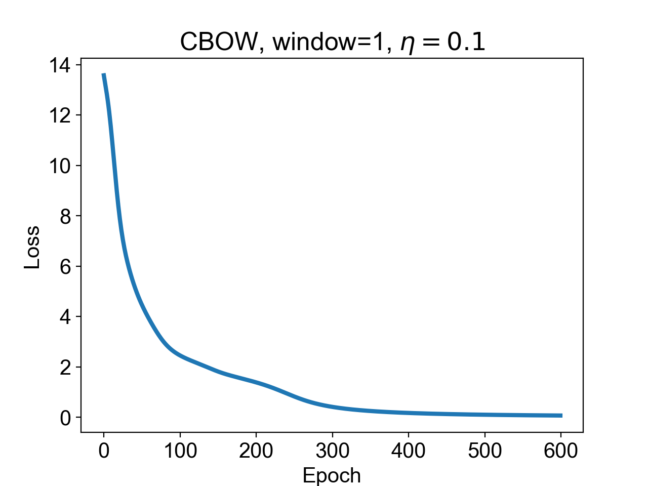
As you can see, the loss function keeps decreasing until almost zero. It does look like the model is working! I am not sure about you, but when I saw this plot I was really curious to see if the weights that the model had learnt were really good at predicting the center words given the context words.
I have added a prediction step in word2veclite that we can use for this purpose. Let’s use it and check, for example, that for the context word “like” - or [0, 1, 0, 0, 0, 0, 0] - the model predicts that the center word is “I” - or [1, 0, 0, 0, 0, 0, 0].
1 | x = np.array([[0, 1, 0, 0, 0, 0, 0]]) |
As you can see, the prediction steps uses the weights W1 and W2 that are learnt from the model. The print statement above outputs the following line:1
prediction_cbow = [9.862e-01, 8.727e-03, 7.444e-09, 5.070e-03, 5.565e-13, 6.154e-10, 7.620e-14]
It works! Indeed, the array above is close to the expected [1, 0, 0, 0, 0, 0, 0].
Let’s try a different example. We take as context words the words “I” and “playing” and we hope to see “like” as the model prediction.1
2
3x = np.array([[1, 0, 0, 0, 0, 0, 0], [0, 0, 1, 0, 0, 0, 0]])
y_pred = cbow.predict(x, W1, W2)
print(("prediction_cbow = [" + 6*"{:.3e}, " + "{:.3e}]").format(*y_pred))
This time the code outputs:1
prediction_cbow = [1.122e-02, 9.801e-01, 8.636e-03, 1.103e-06, 1.118e-06, 1.022e-10, 2.297e-10]
Once again, the prediction is close to the expected center word [0, 1, 0, 0, 0, 0, 0].
Let’s now move to training a Skip-gram model with the same parameters as before. We can do this by simply changing method=”cbow” into method=”skipgram”,1
2
3
4
5
6
7from word2veclite import Word2Vec
corpus = "I like playing football with my friends"
skipgram = Word2Vec(method="skipgram", corpus=corpus,
window_size=1, n_hidden=2,
n_epochs=600, learning_rate=0.1)
W1, W2, loss_vs_epoch = skipgram.run()
This is the loss curve that we get from the code above: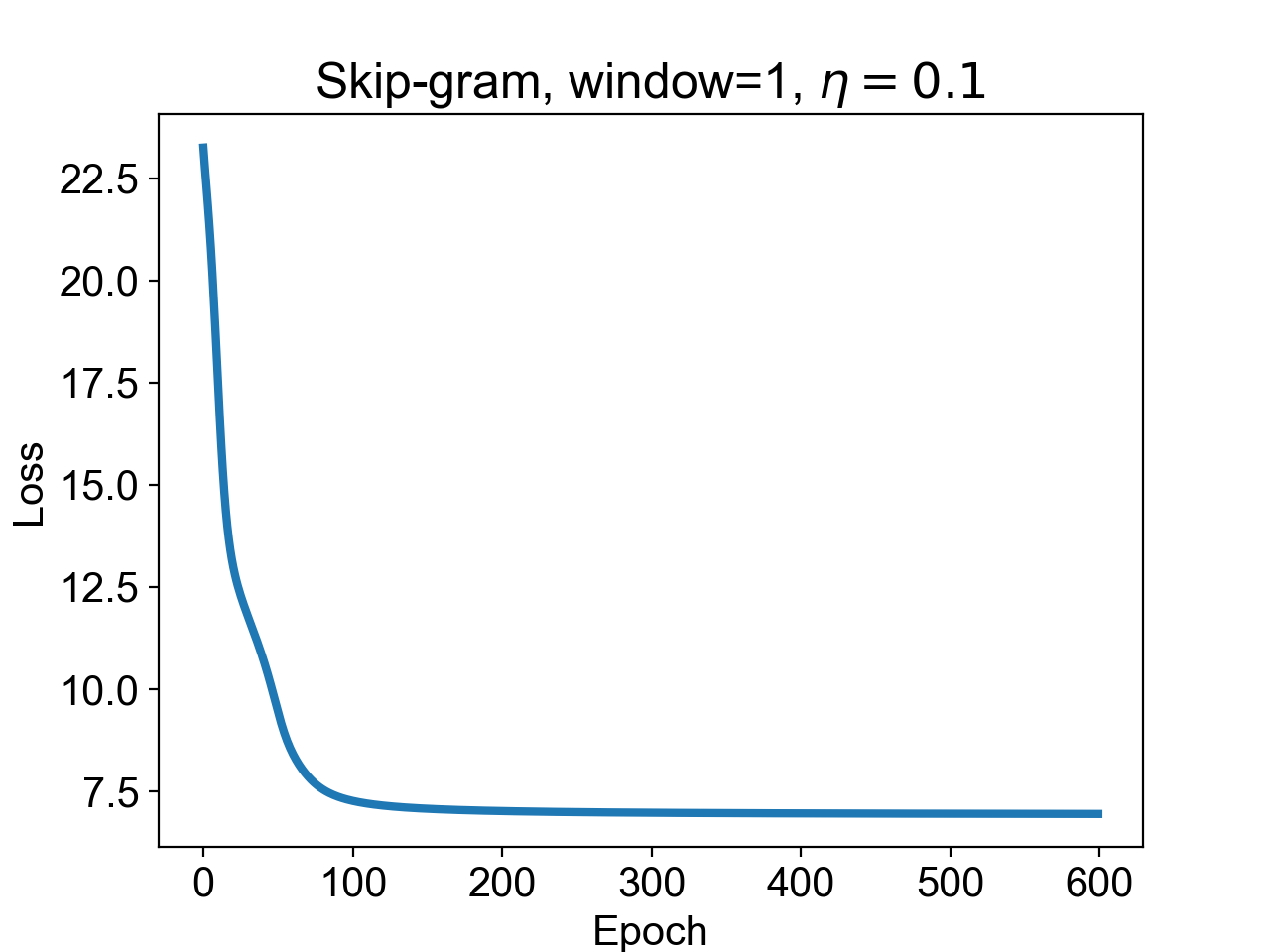
Once again, the model seems to have converged and learnt its weights. To check for this, we look at two more examples. For the center word “I” we expect to see “like” as the context word,
1 | x = np.array([[1, 0, 0, 0, 0, 0, 0]]) |
and this is our prediction:1
prediction_skipgram = [1.660e-03, 9.965e-01, 3.139e-06, 1.846e-03, 1.356e-09, 3.072e-08, 3.146e-10]
which is close to the expected [0, 1, 0, 0, 0, 0, 0].
Our final example now. For the center word “like” we should expected the model to predict the words “I” and “playing” with equal probability.1
2
3x = np.array([[0, 1, 0, 0, 0, 0, 0]])
y_pred = skipgram.predict(x, W1, W2)
print(("prediction_skipgram = [" + 6*"{:.3e}, " + "{:.3e}]").format(*y_pred))
which outputs1
prediction_skipgram = [4.985e-01, 9.816e-04, 5.002e-01, 2.042e-08, 3.867e-04, 3.767e-11, 1.956e-07]
close to the ideal [0.5, 0, 0.5, 0, 0, 0, 0].
This is it for now. I hope you enjoyed the reading!
⁂