Julia has been around since 2012 and after more than six years of development, its 1.0 version has been finally released. This is a major milestone and one that has inspired me to write a new blogpost (after several months of silence). This time we are going to see how to do parallel programming in Julia using the Message Passing Interface (MPI) paradigm, through the open source library Open MPI. We will do this by solving a real physical problem: heat diffusion across a two-dimensional domain.

This is going to be a fairly advanced application of MPI, targeted at someone that has already had some basic exposure to parallel computing. Because of this, I am not going to go step by step but I will rather focus on specific aspects that I feel are of interest (specifically, the use of ghost cells and message passing on a two-dimensional grid). As I have started doing in my recent blogposts, the code discussed here is only partial. It is accompanied by a fully featured solution that you can find on Github and I have named Diffusion.jl.

Parallel computing has entered the “commercial world” over the last few years. It is a standard solution for ETL (Extract-Transform-Load) applications where the problem at hand is embarassingly parallel: each process runs independently from all the others and no network communication is needed (until potentially a final “reduce” step, where each local solution is gathered into a global solution).

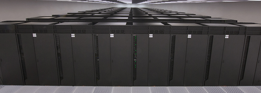
In many scientific applications, there is the need for information to be passed through the network of a cluster. These “non-embarrassingly parallel” problems are often numerical simulations that model problems ranging from astrophysics to weather modelling, biology, quantum systems and many more. In some cases, these simulations are run on tens to even millions of CPUs (Fig. 1) and the memory is distributed - not shared - among the different CPUs. Normally, the way these CPUs communicate in a supercomputer is through the Message Passing Interface (MPI) paradigm.

Anyone working in High Performance Computing should be familiar with MPI. It allows to make use of the architecture of a cluster at a very low level. In theory, a researcher could assign to every single CPU its computational load. He/She could decide exactly when and what information should be passed among CPUs and whether this should happen sinchronously or asynchronously.

And now, let’s go back to the contents of this blogpost, where we are going to see how to write the solution of a diffusion-type equation using MPI. We have already discussed the explicit scheme for a one-dimensional equation of this type. However, in this blogpost we will look at the two-dimensional solution.

The Julia code presented here is essentially a translation of the C/Fortran code explained in this excellent blogpost by Fabien Dournac.

In this blogpost I am not going to present a thorough analysis of scaling speed vs. number of processors. Mainly because I only have two CPUs that I can play with at home (Intel Core i7 processor on my MacBook Pro)… Nonetheless, I can still proudly say that the Julia code presented in this blogpost shows a significant speedup using two CPUs vs. one. Not only this: it is faster than the Fortran and C equivalent codes! (more on this later)

These are the topics that we are going to cover in this blogpost:

• Julia: My first impressions
• How to install Open MPI on your machine
• The problem: diffusion across a two-dimensional domain
• Communication among CPUs: the need for ghost cells
• Using MPI
• Visualizing the solution
• Performance
• Conclusions

1. First impressions about Julia

I am actually still a newbie with Julia, hence the choice of having a secion on my “first impressions”.

The main reason why I got interested in Julia is that it promises to be a general purpose framework with a performance comparable to the likes of C and Fortran, while keeping the flexibility and ease of use of a scripting language like Matlab or Python. In essence, it should be possible to write Data Science/High-Performance-Computing applications in Julia that run on a local machine, on the cloud or on institutional supercomputers.

One aspect I don’t like is the workflow, which seems sub-optimal for someone like me that uses IntelliJ and PyCharm on a daily basis (the IntelliJ Julia plugin is terrible). I have tried the Juno IDE as well, it is probably the best solution at the moment but I still need to get used to it.

One aspect that demonstrates how Julia has still not reached its “maturity” is how varied and outdated is the documentation of many packages. I still haven’t found a way to write a matrix of Floating point numbers to disk in a formatted way. Sure, you can write to disk each element of the matrix in a double-for loop but there should be better solutions available. It is simply that information can be hard to find and the documentation is not necessarily exhaustive.

Another aspect that stands out when first using Julia is the choice of using one-based indexing for arrays. While I find this slightly annoying from a practical perspective, it is surely not a deal breaker also considering that this not unique to Julia (Matlab and Fortran use one-based indexing, too).

Now, to the good and most important aspect: Julia can indeed be really fast. I was impressed to see how the Julia code that I wrote for this blogpost can perform better than the equivalent Fortran and C code, despite having essentially just translated it into Julia. Have a look at the performance section if you are curious.

2. Installing Open MPI

Open MPI is an open source Message Passing Interface library. Other famous libraries include MPICH and MVAPICH. MVAPICH, developed by the Ohio State University, seems to be the most advanced library at the moment as it can also support clusters of GPUs - something particularly useful for Deep Learning applications (there is indeed a close collaboration between NVIDIA and the MVAPICH team).

All these libraries are built on a common interface: the MPI API. So, it does not really matter whether you use one or the other library: the code you have written can stay the same.

The MPI.jl project on Github is a wrapper for MPI. Under the hood, it uses the C and Fortran installations of MPI. It works perfectly well, although it lacks some functionality that is available in those other languages.

In order to be able to run MPI in Julia you will need to install separately Open MPI on your machine. If you have a Mac, I found this guide to be very useful. Importantly, you will need to have also gcc (the GNU compiler) installed as Open MPI requires the Fortran and C compilers. I have installed the 3.1.1 version of Open MPI, as mpiexec --version on my Terminal also confirms.

Once you have Open MPI installed on your machine, you should install cmake. Again, if you have a Mac this is as easy as typing brew install cmake on your Terminal.

At this point you are ready to install the MPI package in Julia. Open up the Julia REPL and type Pkg.add(“MPI”). Normally, at this point you should be able to import the package using import MPI. However, I also had to build the package through Pkg.build(“MPI”) before everything worked.

3. The problem: diffusion in a two-dimensional domain

The diffusion equation is an example of a parabolic partial differential equation. It describes phenomena such as heat diffusion or concentration diffusion (Fick’s second law). In two spatial dimensions, the diffusion equation writes

The solution $u(x, y, t)$ represents how the temperature/concentration (depending on whether we are studying heat or concentration diffusion) varies in space and time. Indeed, the variables $x, y$ represent the spatial coordinates, while the time component is represented by the variable $t$. The quantity $D$ is the “diffusion coefficient” and determines how fast heat, for example, is going to diffuse through the physical domain. Similarly to what was discussed (in more detail) in a previous blogpost, the equation above can be discretized using a so-called “explicit scheme” of solution. I am not going to go through the details here, that you can find in said blogpost, it suffices to write down the numerical solution in the following form,
$$\begin{equation} \frac{u_{i,k}^{j+1} - 2u_{i,k}^{j}}{\Delta t} = D\left(\frac{u_{i+1,k}^j-2u_{i,k}^j+u_{i-1,k}^j}{\Delta x^2}+ \frac{u_{i,k+1}^j-2u_{i,k}^j+u_{i,k-1}^j}{\Delta y^2}\right) \label{eq:diffusion} \end{equation}$$
where the $i, k$ indices refer to the spatial grid while $j$ represents the time index.
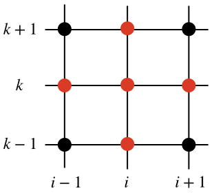
Assuming all the quantities at the time $j$ to be known, the only unknown is $u_{i,k}^{j+1}$ on the left hand side of eq. (\ref{eq:diffusion}). This quantity depends on the values of the solution at the previous time step $j$ in a cross-shaped stencil, as in the figure below (the red dots represent those grid points at the time step $j$ that are needed in order to find the solution $u_{i,k}^{j+1}$).

Equation (\ref{eq:diffusion}) is really all is needed in order to find the solution across the whole domain at each subsequent time step. It is rather easy to implement a code that does this sequentially, with one process (CPU). However, here we want to discuss a parallel implementation that uses multiple processes.

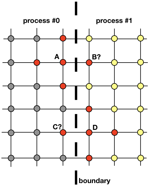
Each process will be responsible for finding the solution on a portion of the entire spatial domain. Problems like heat diffusion, that are not embarrassingly parallel, require exhchanging information among the processes. To clarify this point, let’s have a look at Figure 3. It shows how processes #0 and #1 will need to communicate in order to evaluate the solution near the boundary. This is where MPI enters. In the next section, we are going to look at an efficient way of communicating.

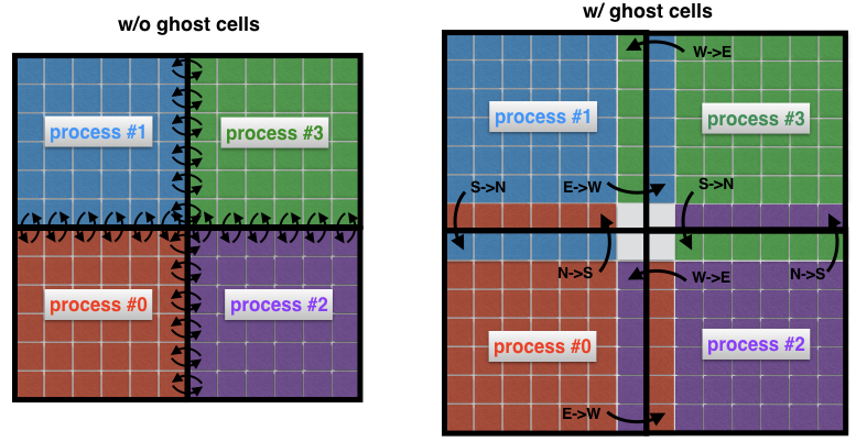
4. Communication among processes: ghost cells

An important notion in computational fluid dynamics is the one of ghost cells. This concept is useful whenever the spatial domain is decomposed into multiple sub-domains, each of which is solved by one process.

In order to understand what ghost cells are, let’s consider again the two neighboring regions depicted in Figure 3. Process #0 is responsible for finding the solution on the left hand side, whereas process #1 finds it on the right hand side of the spatial domain. However, because of the shape of the stencil (Fig. 2), near the boundary both processes will need to communicate between them. Here is the problem: it is very inefficient to have process #0 and process #1 communicate each time they need a node from the neighboring process: it would result in an unacceptable communication overhead.

Instead, what is common practice is to surround the “real” sub-domains with extra cells called ghost cells, as in Figure 4 (right). These ghost cells represent copies of the solution at the boundaries of neighboring sub-domains. At each time step, the old boundary of each sub-domain is passed to its neighbors. This allows the new solution at the boundary of a sub-domain to be calculated with a significantly reduced communication overhead. The net effect is a speedup in the code.

5. Using MPI

There are a lot of tutorials on MPI. Here, I just want to describe those commands - expressed in the language of the MPI.jl wrapper for Julia - that I have been using for the solution of the 2D diffusion problem. They are some basic commands that are used in virtually every MPI implementation.

5.1 Finding the neighbors of a process

For our problem, we are going to decompose our two-dimensional domain into many rectangular sub-domains, similar to the Figure below

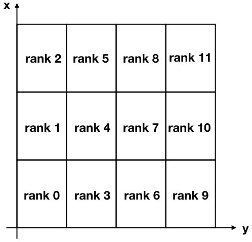
Note that the “x” and “y” axis are flipped with respect to the conventional usage, in order to associate the x-axis to the rows and the y-axis to the columns of the matrix of solution.

In order to communicate between the various processes, each process needs to know what its neighbors are. There is a very convenient MPI command that does this automatically and is called MPI_Cart_create. Unfortunately, the Julia MPI wrapper does not include this “advanced” command (and it does not look trivial to add it), so instead I decided to build a function that accomplishes the same task. In order to make it more compact, I have made extensive use of the ternary operator. You can find this function below,

1
2
3
4
5
6
7
8
9
10
11
12
13
14
15
16
17
18
19
20
21
22
23
24
25

function neighbors(my_id::Int, nproc::Int, nx_domains::Int, ny_domains::Int)
    id_pos = Array{Int,2}(undef, nx_domains, ny_domains)
    for id = 0:nproc-1
        n_row = (id+1) % nx_domains > 0 ? (id+1) % nx_domains : nx_domains
        n_col = ceil(Int, (id + 1) / nx_domains)
        if (id == my_id)
            global my_row = n_row
            global my_col = n_col
        end
        id_pos[n_row, n_col] = id
    end

    neighbor_N = my_row + 1 <= nx_domains ? my_row + 1 : -1
    neighbor_S = my_row - 1 > 0 ? my_row - 1 : -1
    neighbor_E = my_col + 1 <= ny_domains ? my_col + 1 : -1
    neighbor_W = my_col - 1 > 0 ? my_col - 1 : -1

    neighbors = Dict{String,Int}()
    neighbors["N"] = neighbor_N >= 0 ? id_pos[neighbor_N, my_col] : -1
    neighbors["S"] = neighbor_S >= 0 ? id_pos[neighbor_S, my_col] : -1
    neighbors["E"] = neighbor_E >= 0 ? id_pos[my_row, neighbor_E] : -1
    neighbors["W"] = neighbor_W >= 0 ? id_pos[my_row, neighbor_W] : -1

    return neighbors
end

The inputs of this function are my_id, which is the rank (or id) of the process, the number of processes nproc, the number of divisions in the $x$ direction nx_domains and the number of divisions in the $y$ direction ny_domains.

Let’s now test this function. For example, looking again at Fig. 5, we can test the output for process of rank 4 and for process of rank 11. This is what we find on a Julia REPL:

1
2
3
4
5
6

julia> neighbors(4, 12, 3, 4)
Dict{String,Int64} with 4 entries:
  "S" => 3
  "W" => 1
  "N" => 5
  "E" => 7

1
2
3
4
5
6

julia> neighbors(11, 12, 3, 4)
Dict{String,Int64} with 4 entries:
  "S" => 10
  "W" => 8
  "N" => -1
  "E" => -1

As you can see, I am using cardinal directions “N”, “S”, “E”, “W” to denote the location of a neighbor. For example, process #4 has process #3 as a neighbor located South of its position. You can check that the above results are all correct, given that “-1” in the second example means that no neighbors have been found on the “North” and “East” sides of process #11.

5.2 Message passing

As we have seen earlier, at each iteration every process sends its boundaries to the neighboring processes. At the same time, every process receives data from its neighbors. These data are stored as “ghost cells” by each process and are used to compute the solution near the boundary of each sub-domain.

There is a very useful command in MPI called MPI_Sendrecv that allows to send and receive messages at the same time, between two processes. Unfortunately MPI.jl does not provide this functionality, however it is still possible to achieve the same result by using the MPI_Send and MPI_Receive functionalities separately.

This is what is done in the following updateBound! function, which updates the ghost cells at each iteration. The inputs of this function are the global 2D solution u, which includes the ghost cells, as well as all the information related to the specific process that is running the function (what its rank is, what are the coordinates of its sub-domain, what are its neighbors). The function first sends its boundaries to its neighbors and then it receives their boundaries. The receive part is finalized through the MPI.Waitall! command, that ensures that all the expected messages have been received before updating the ghost cells for the specific sub-domain of interest.

1
2
3
4
5
6
7
8
9
10
11
12
13
14
15
16
17
18
19
20
21
22
23
24
25
26
27
28
29
30
31
32
33
34
35
36
37
38
39
40
41
42
43
44
45
46
47
48
49
50
51
52
53
54
55
56

function updateBound!(u::Array{Float64,2}, size_total_x, size_total_y, neighbors, comm,
                       me, xs, ys, xe, ye, xcell, ycell, nproc)

    mep1 = me + 1

    #assume, to start with, that this process is not going to receive anything
    rreq = Dict{String, MPI.Request}(
                                "N" => MPI.REQUEST_NULL,
                                "S" => MPI.REQUEST_NULL,
                                "E" => MPI.REQUEST_NULL,
                                "W" => MPI.REQUEST_NULL
                                )
    recv = Dict{String, Array{Float64,1}}()
    ghost_boundaries = Dict{String, Any}(
                                "N" => (xe[mep1]+1, ys[mep1]:ye[mep1]),
                                "S" => (xs[mep1]-1, ys[mep1]:ye[mep1]),
                                "E" => (xs[mep1]:xe[mep1], ye[mep1]+1),
                                "W" => (xs[mep1]:xe[mep1], ys[mep1]-1)
                                )
    is_receiving = Dict{String, Bool}("N" => false, "S" => false, "E" => false, "W" => false)

    #send
    neighbors["N"] >=0 && MPI.Isend(u[xe[mep1], ys[mep1]:ye[mep1]], neighbors["N"], me + 40, comm)
    neighbors["S"] >=0 && MPI.Isend(u[xs[mep1], ys[mep1]:ye[mep1]], neighbors["S"], me + 50, comm)
    neighbors["E"] >=0 && MPI.Isend(u[xs[mep1]:xe[mep1], ye[mep1]], neighbors["E"], me + 60, comm)
    neighbors["W"] >=0 && MPI.Isend(u[xs[mep1]:xe[mep1], ys[mep1]], neighbors["W"], me + 70, comm)

    #receive
    if (neighbors["N"] >= 0)
        recv["N"] = Array{Float64,1}(undef, ycell)
        is_receiving["N"] = true
        rreq["N"] = MPI.Irecv!(recv["N"], neighbors["N"], neighbors["N"] + 50, comm)
    end
    if (neighbors["S"] >= 0)
        recv["S"] = Array{Float64,1}(undef, ycell)
        is_receiving["S"] = true
        rreq["S"] = MPI.Irecv!(recv["S"], neighbors["S"], neighbors["S"] + 40, comm)
    end
    if (neighbors["E"] >= 0)
        recv["E"] = Array{Float64,1}(undef, xcell)
        is_receiving["E"] = true
        rreq["E"] = MPI.Irecv!(recv["E"], neighbors["E"], neighbors["E"] + 70, comm)
    end
    if (neighbors["W"] >= 0)
        recv["W"] = Array{Float64,1}(undef, xcell)
        is_receiving["W"] = true
        rreq["W"] = MPI.Irecv!(recv["W"], neighbors["W"], neighbors["W"] + 60, comm)
    end

    MPI.Waitall!([rreq[k] for k in keys(rreq)])
    for (k, v) in is_receiving
        if v
            u[ghost_boundaries[k][1], ghost_boundaries[k][2]] = recv[k]
        end
    end
end

5. Visualizing the solution

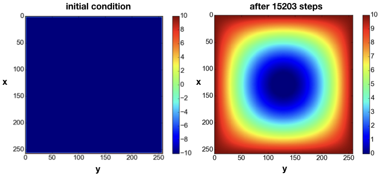
The domain is initialized with a constant value $u=+10$ around the boundary, which can be interpreted as having a source of constant temperature at the border. The initial condition is $u=-10$ in the interior of the domain (Fig. 6left). As time progresses, the value $u=10$ at the boundary diffuses towards the center of the domain. For example, at the time step j=15203, the solution looks like as in Fig. 6right.

As the time $t$ increases, the solution becomes more and more homogenous, until theoretically for $t \rightarrow +\infty$ it becomes $u=+10$ across the entire domain.

6. Performance

I was very impressed when I tested the performance of the Julia implementation against Fortran and C: I found the Julia implementation to be the fastest one!

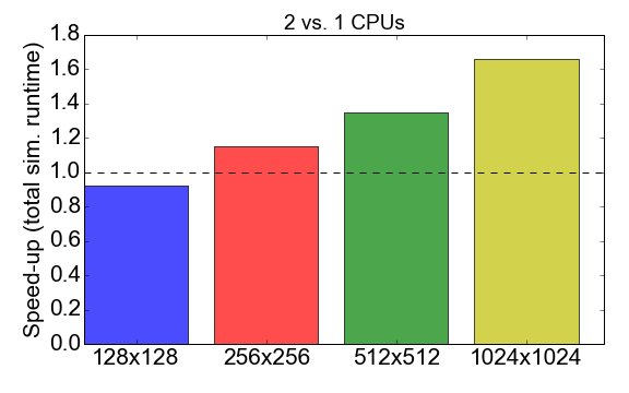
Before jumping into this comparison, let’s have a look at the MPI performance of the Julia code itself. Figure 7 shows the ratio of the runtime when running with 1 vs. 2 processes (CPUs). Ideally, you would like this number to be close to 2, i.e., that running with 2 CPUs should be twice as fast than running with one CPU. What is observed instead is that for small problem sizes (grid of 128x128 cells), the compilation time and communication overhead have a net negative effect on the overall runtime: the speed-up is smaller than one. It is only for larger problem sizes that the benefit of using multiple processes starts to be apparent.

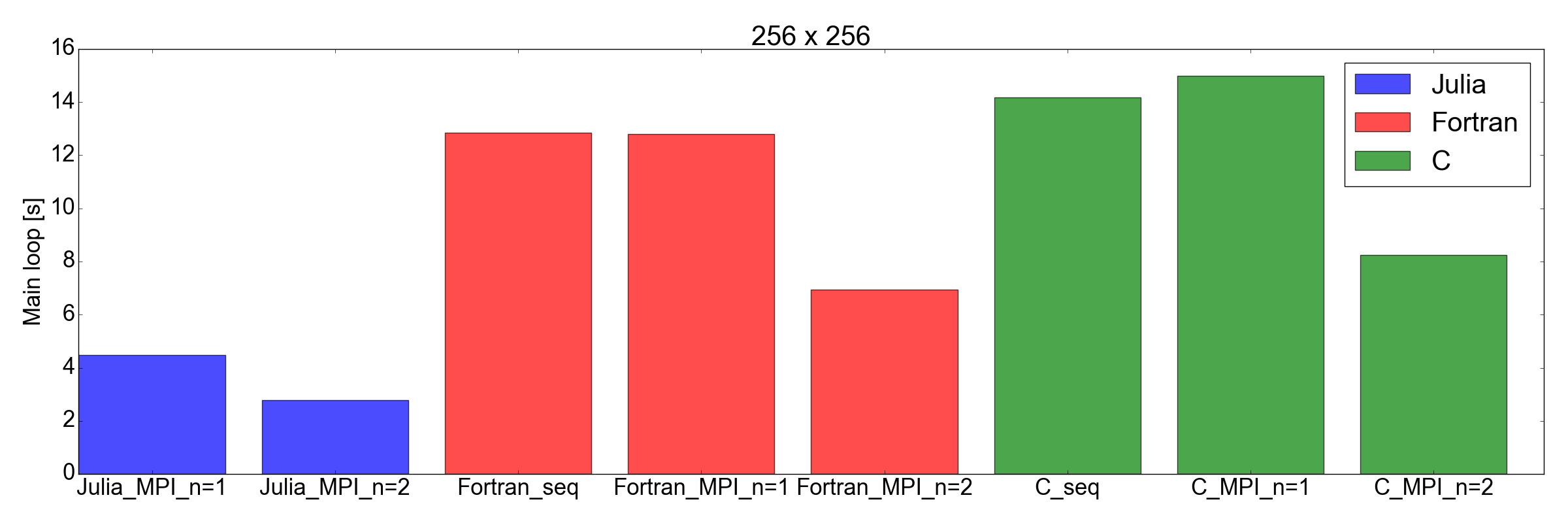
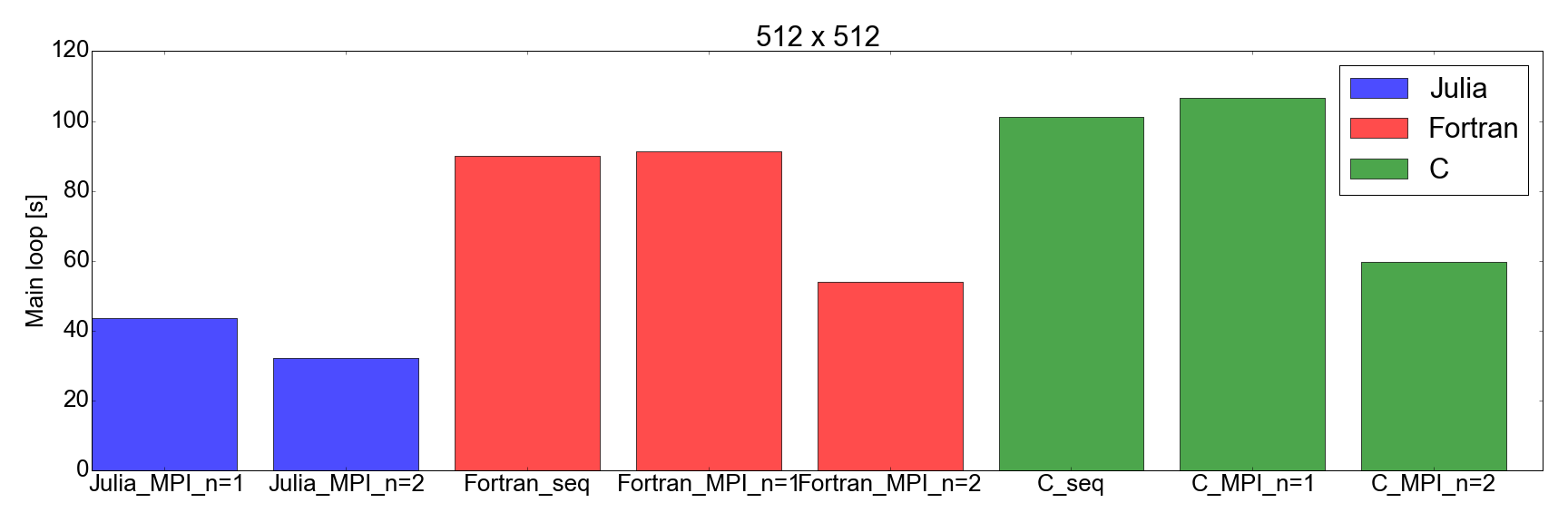
And now, for the surprise plot: Fig. 8 demonstrates that the Julia implementation is faster than both Fortran and C, for both 256x256 and 512x512 problem sizes (the only ones I tested). Here I am only measuring the time needed in order to complete the main iteration loop. I believe this is a fair comparison, as for long running simulations this is going to represent the biggest contribution to the total runtime.

Conclusions

Before starting this blogpost I was fairly skeptical of Julia being able to compete against the speed of Fortran and C for scientific applications. The main reason was that I had previously translated an academic code of about 2000 lines from Fortran into Julia 0.6 and I observed a performance reduction of about x3.

But this time… I am very impressed. I have effectively just translated an existing MPI implementation written in Fortran and C, into Julia 1.0. The results shown in Fig. 8 speak for themselves: Julia appears to be the fastest by far. Note that I have not factored in the long compilation time taken by the Julia compiler, as for “real” applications that take hours to complete this would represent a negligible factor.

I should also add that my tests are surely not as exhaustive as they should be for a thorough comparison. In fact, I would be curious to see how the code performs with more than just 2 CPUs (I am limited by my home personal laptop) and with different hardware (feel free to check out Diffusion.jl!).

At any rate, this exercise has convinced me that it is worth investing more time in learning and using Julia for Data Science and scientific applications. Off to the next one!

References

Fabien Dournac, Version MPI du code de résolution numérique de l’équation de chaleur 2D