This article started as an excuse to present a Python code that solves a one-dimensional diffusion equation using finite differences methods. I then realized that it did not make much sense to talk about this problem without giving more context so I finally opted for writing a longer article. I have divided this article into three posts, of which this is the first one.

The first two blog posts (including this one) are dedicated to some basic theory on how to numerically solve parabolic partial differential equations (PDEs). The third blog post will be dedicated to showing a short python code that solves one particular parabolic problem.

Below is a list of the topics of this blog post

• a short introduction to parabolic PDEs
• the basics for solving PDEs: finite difference methods
• the simplest algorithm of solution: explicit solution
• stability constraints (or, when does the explicit solution fail?)

1. Parabolic PDEs

Parabolic partial differential equations model important physical phenomena such as heat conduction (described by the heat equation) and diffusion (for example, Fick’s law). Under an appropriate transformation of variables the Black-Scholes equation can also be cast as a diffusion equation. I might actually dedicate a full post in the future to the numerical solution of the Black-Scholes equation, that may be a good idea…

The simplest parabolic problem is of the type
\begin{equation}
\frac{\partial u}{\partial t} = D\frac{\partial^2 u}{\partial x^2} \ + \mathrm{I.B.C.}
\label{eq:diffusion}
\end{equation}

where $D$ is a diffusion/heat coefficient (for simplicity, assumed to be independent of the time $t$ and space $x$ variables) and I.B.C. stands for “initial and boundary conditions”. The unknown $u$ represents a generic quantity of interest, which depends on the specific problem (could be temperature, concentration, price of an option,…).

The boundary conditions specify the constraints that the solution has to fulfill at the boundaries of the domain of interest. For example, let’s assume we have to solve a problem of heat conduction along a metallic rod as in the figure below. We keep the two sides of the rod at a fixed temperature $T^*$ and the initial temperature profile inside the domain is given by a function $T_0(x)$, which in general is dependent on the coordinate $x$.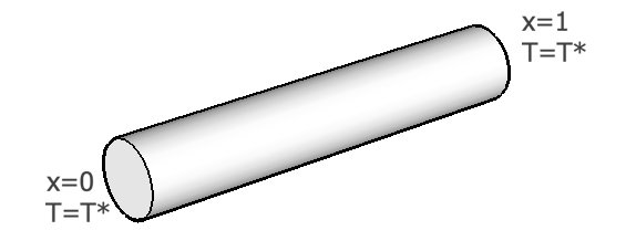

This problem can be well approximated by a 1D model of heat conduction (as we assume that the length of the rod is much larger than the dimensions of its section). For simplicity, let’s assume $D=1$ in eq. (\ref{eq:diffusion}). The heat diffusion problem requires then to find a function $T(x,t)$ that satisfies the following equations

$$\left\{ \begin{eqnarray} \frac{\partial T}{\partial t} \ \ &=& \ \frac{\partial^2 T}{\partial x^2} \ \ & 0< x <1 \nonumber \\ T(0,t) &=& T(1,t) \ = T^* & \ \ \ \ \ \ \forall t\nonumber\\ T(x,0) &=& T_0(x) & 0<x<1 \nonumber \end{eqnarray} \right.$$

where this time I have explicitly written the initial and boundary conditions. This is now a well defined problem that can be solved numerically.

The numerical solution involves writing approximate expressions for the derivatives above, via a method called finite differences, that I describe briefly below.

2. Finite differences

Derivatives, such as the quantities $\partial u/\partial t$ and $\partial^2 u/\partial x^2$ that appear in eq. ($\ref{eq:diffusion}$), are a mathematical abstraction that can only be approximated when using numerical techniques.

Going back to the very definition of the derivative of a one-dimensional function $f(x)$, the derivative $f’(x)$ of this function at the point $x$ is defined as

$$\begin{equation} f'(x) = \underset{\Delta x\rightarrow 0}\lim\frac{f(x+\Delta x)-f(x)}{\Delta x} = \underset{\Delta x\rightarrow 0}\lim\frac{\Delta f}{\Delta x} \end{equation}$$

Now, while a CPU can easily calculate the differences $\Delta f$ and $\Delta x$, it is a different story to calculate the limit $\lim(\Delta x\rightarrow 0)$. That is not a basic arithmetic operation. So, how to calculate the derivative? The trick is to calculate the ratio $\Delta f/\Delta x$ for a “sufficiently small” value of $\Delta x$. We can in fact approximate the derivative in different ways, making use of Taylor’s theorem

$$\begin{eqnarray} f(x+\Delta x) = f(x) + f'(x)\Delta x + \frac{1}{2}f''(x)\Delta x^2 + \frac{1}{6}f'''(x)\Delta x^3 + \dots \label{eq:taylor1}\\ f(x-\Delta x) = f(x) - f'(x)\Delta x + \frac{1}{2}f''(x)\Delta x^2 - \frac{1}{6}f'''(x)\Delta x^3 + \dots \label{eq:taylor2} \end{eqnarray}$$

Summing up the two equations above, we get
$$\begin{equation} f(x+\Delta x) + f(x-\Delta x) = 2f(x) + f''(x)\Delta x^2 + O(\Delta x^4), \end{equation}$$
where $O(\Delta x^4)$ indicates terms containing fourth and higher order powers of $\Delta x$ (negligible with respect to lower powers of $\Delta x$ for $\Delta x \rightarrow 0$).

This immediately gives us an expression for the second derivative $f’’(x)$,
$$\begin{equation} f''(x) = \frac{f(x+\Delta x)-2f(x)+f(x-\Delta x)}{\Delta x^2} + O(\Delta x^4) \label{eq:fd1} \end{equation}$$
and for the approximation that is suited for calculations using a CPU,
$$\begin{equation} \bbox[lightblue,5px,border:2px solid red]{f''(x) \simeq \frac{f(x+\Delta x)-2f(x)+f(x-\Delta x)}{\Delta x^2}} \label{eq:fd2} \end{equation}$$
Similarly, subtraction of eq. (\ref{eq:taylor2}) from eq. (\ref{eq:taylor1}) leads to the central-difference approximation to the first derivative,
$$\begin{equation} \bbox[lightblue,5px,border:2px solid red]{f'(x) \simeq \frac{f(x+\Delta x)-f(x-\Delta x)}{2\Delta x}} \label{eq:fd3} \end{equation}$$
with an error $O(\Delta x^2)$. Alternative approximations to the first derivative are the forward-difference formula,
$$\begin{equation} \bbox[lightblue,5px,border:2px solid red]{f'(x) \simeq \frac{f(x+\Delta x)-f(x)}{\Delta x}} \label{eq:fd4} \end{equation}$$
with an error $O(\Delta x)$, and the backward-difference formula
$$\begin{equation} \bbox[lightblue,5px,border:2px solid red]{f'(x) \simeq \frac{f(x)-f(x-\Delta x)}{\Delta x}} \label{eq:fd5} \end{equation}$$
also with an error $O(\Delta x)$.

Higher order (or mixed) derivatives can be calculated in a similar fashion. The important point is that the approximations (\ref{eq:fd2},\ref{eq:fd3},\ref{eq:fd4},\ref{eq:fd5}) form the building blocks for the numerical solution of ordinary and partial differential equations.

In the next section I will discuss a first algorithm that uses these approximations to solve eq. ($\ref{eq:diffusion}$) and goes under the name of explicit solution. It is a fast and intuitive algorithm, that however has the drawback of only working under some well defined conditions, otherwise the solution is unstable (i.e., the numerical solution will get NaN values pretty quickly…).

3. Explicit solution to the diffusion equation

Let’s go back to eq. ($\ref{eq:diffusion}$) and think about a possible way of solving this problem numerically. Using the results of the previous section, we can think of discretizing the derivative $\partial u/\partial t$ using any of the formulas above (central/forward/backward differencing) and the derivative $\partial u^2/\partial x^2$ using eq. (\ref{eq:fd2}). As it turns out, for stability considerations it is better to avoid central differencing for $\partial u/\partial t$. We will use instead forward differencing (we could also choose backward differencing), and the fully discretized equation then looks like
$$\begin{equation} \frac{u_{i,j+1}-u_{i,j}}{\Delta t} = D\frac{u_{i+1,j}-2u_{i,j}+u_{i-1,j}}{\Delta x^2}, \label{eq:fd} \end{equation}$$
to which the initial and boundary conditions need to be added.

Note how eq. (\ref{eq:fd}) implies having already defined a space and time grids. Let’s assume the spatial resolution is $\Delta x$ and the temporal resolution is $\Delta t$. Then if $u(i,j)$ is the solution at the position $x$ and time $t$, $u(i+1,j+1)$ represents the solution at the position $x+\Delta x$ and at the time $t + \Delta t$. Visually, the space-time grid can be seen in the figure below.

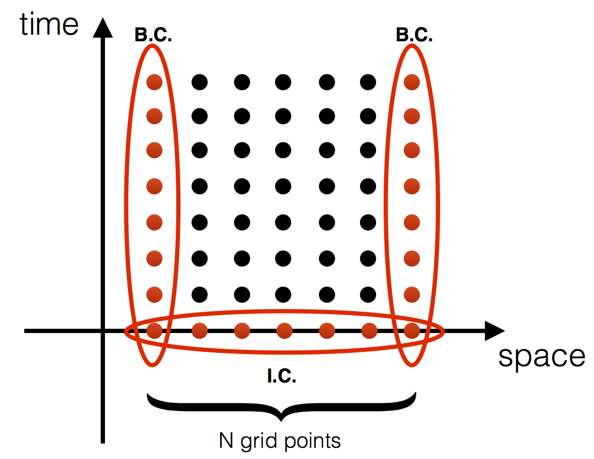
The initial and boundary conditions are represented by red dots in the figure. The space grid is represented by the index $i$ in eq. (\ref{eq:fd}), while the time is represented by the index $j$. At the beginning of the simulation, the space domain is discretized into $N$ grid points, so that $i=1\dots N$. The index $j$ starts from $j=1$ (the initial condition) and runs for as long as needed to capture the dynamics of interest.

Looking at the figure above, it is clear that the only unknown in eq. (\ref{eq:fd}) is $u_{i,j+1}$. Solving for this quantity, we get
$$\begin{equation} u_{i,j+1} = r\,u_{i+1,j} + (1-2r)u_{i,j} + r\,u_{i-1,j} \label{eq:explicit} \end{equation}$$
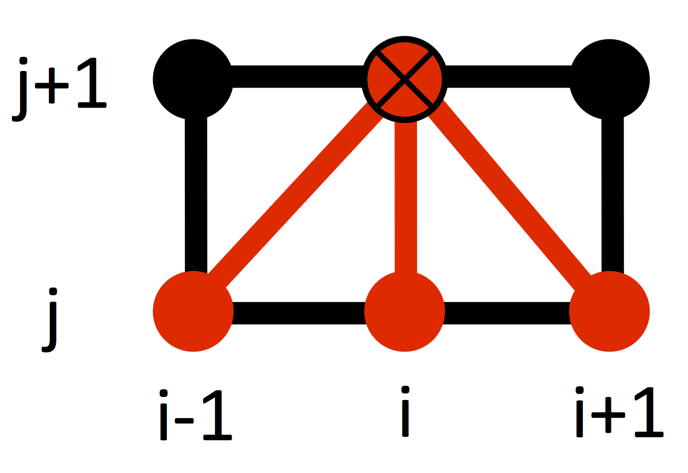
where $r = D\Delta t/\Delta x^2$. As shown in Figure 3, the unknown $u_{i,j+1}$ only depends on quantities at the previous time step $j$, and only at the grid points $i-1, i$ and $i+1$.

Equation (\ref{eq:explicit}) can be recast in matrix form. Remember that the boundary conditions are given at the gridpoints $i=1$ and $i=N$, so the real unknowns are the values at the gridpoints $i=2,\dots,N-1$ and at the timestep $j+1$, giving

$$\begin{equation} \left( \begin{matrix} u_{2,j+1} \\ u_{3,j+1} \\ \vdots \\ u_{N-2,j+1} \\ u_{N-1,j+1} \\ \end{matrix} \right) = \left( \begin{matrix} 1-2r & r & & & \\ r & 1-2r & r & \Huge{0} &\\ & & \ddots & & & \\ & \Huge{0} & r & 1-2r & r \\ & & & r & 1-2r \\ \end{matrix} \right) \left( \begin{matrix} u_{2,j} \\ u_{3,j} \\ \vdots \\ u_{N-2,j} \\ u_{N-1,j} \\ \end{matrix} \right) + \left( \begin{matrix} r u_{1,j} \\ 0 \\ \vdots \\ 0 \\ r u_{N,j} \\ \end{matrix} \right) \label{eq:matrix1} \end{equation}$$

which can be rewritten as

$$\begin{equation} \textbf{u}_{j+1} = B\textbf{u}_{j} + \textbf{b}_{j}. \label{eq:matrix2} \end{equation}$$

where $B$ is a square $(N-1)\times (N-1)$ matrix and $\textbf{b}_{j}$ is a vector of boundary conditions. The matrix $B$ is tri-diagonal.

It is pretty easy to implement the solution (\ref{eq:matrix2}) in a code, but there is a potential big problem that we should be aware of when using this type of algorithm (explicit): the solution can be unstable! This means that any small and unavoidable round-off error can degenerate to a huge error (and eventually NaNs) after a few hundreds or thousands of iterations.

How can we make sure we don’t suffer from this problem? That’s the subject of the next section.

2.1 Stability condition

Equation ($\ref{eq:matrix2}$) is only an approximate solution of eq. ($\ref{eq:diffusion}$). In fact, it is not even possible to solve exactly eq. ($\ref{eq:matrix2}$), let alone eq. (\ref{eq:diffusion}), because of round-off errors. How can we guarantee that these initially small errors will not accumulate over many iterations causing a catastrophic runtime error during execution of our code?

Let’s do a direct calculation: let’s assume that the true solution of ($\ref{eq:matrix2}$) - which as noted is already an approximation of the original problem - is given by the quantity $\textbf{u}_1$, while due to roundoff-errors our code finds the solution $\textbf{u}_1^*$. What is going to happen to the error $\textbf{e}_1 = \textbf{u}_1 - \textbf{u}_1^*$? Is it going to be amplified at successive iterations, or will it always be possible to bound the propagated error by some number independent of the iteration step $j$?

To answer this question, we can apply recursively eq. (\ref{eq:matrix2}) to find

$$\begin{eqnarray} \textbf{u}_j=B^j\textbf{u}_1+B^{j-1}\textbf{b}_1+\dots+B^{j-2}\textbf{b}_2+\textbf{b}_{j} \\ \textbf{u}^*_j=B^j\textbf{u}^*_1+B^{j-1}\textbf{b}_1+\dots+B^{j-2}\textbf{b}_2+\textbf{b}_{j} \end{eqnarray}$$

where $B^j=B\times B\dots \times B$ ($j$ times). It follows that at the timestep $j$ the difference of the solutions will be $$\textbf{e}_j=\textbf{u}_j-\textbf{u}^*_j=B^j \textbf{e}_1,$$
which implies
$$||\textbf{e}_j||\leq||B^j||\,||\textbf{e}_1||\ .$$

According to Lax and Ritchmyer, for the numerical scheme to be stable there should exist a positive number M independent of $j, \Delta x$ and $\Delta t$ such that $||B^j||\leq M \ \forall \ j\ $, so that

$$\begin{equation} ||\textbf{e}_j||\leq M ||\textbf{e}_1||\ . \label{eq:lax-ritchmyer} \end{equation}$$

This ensures that a small error at the first timestep, $\textbf{e}_1$, will not propagate catastrophically at subsequent timesteps.

The necessary and sufficient condition for the Lax-Ritchmyer stability condition (\ref{eq:lax-ritchmyer}) to be satisfied is $||B||\leq 1$. For the explicit method of eqs. (\ref{eq:matrix1}) and (\ref{eq:matrix2}), it can be shown that a sufficient condition to guarantee that $||B||\leq 1$ is

$$r\leq \frac{1}{2}$$

which, remembering that $r = D\Delta t/\Delta x^2$, translates into
$$\begin{equation} \bbox[lightblue,5px,border:2px solid red]{\Delta t \leq \frac{\Delta x^2}{2D}\ .} \label{eq:stability} \end{equation}$$

Unfortunately, in many practical applications it is not possible to satisfy eq. (\ref{eq:stability}) without strongly compromising the efficiency of an algorithm. For example during the implosion of deuterium (D) and tritum (T) spherical pellets in inertial confinement fusion (ICF) experiments, the D and T ions are subject to mass diffusion (à la Fick). The variable $u$ of eq. (\ref{eq:diffusion}) is in this case the species concentration. In particular conditions the diffusion coefficient $D$ may reach very large values, on the order of $10^2$ m$^2/$s. Now, usually in ICF simulations the grid size is constrained to resolve distances on the order of a $\mu$m (i.e., $\Delta x \sim 10^{-6}$ m). Applying eq. (\ref{eq:stability}), we see that to guarantee stability with an explicit scheme the time step would need to be kept to values $\Delta t\sim 10 $ fs or $10^{-14}$s. Typical ICF codes run with time steps on the order of $10^{-12}$ s. If we were to model species diffusion with an explicit scheme, we would then slow down an ICF code by 2 orders of magnitude (!!).

Is it possible to avoid having a time step constrained by the condition (\ref{eq:stability})? Yes, luckily it is. We need to use a different scheme of solution called implicit. This comes at the price of having to solve a set of equations that is numerically more demanding. We will see in the next post of the series how a popular implicit scheme (Crank-Nicolson) works.

Today’s Mondrian random generator