I must admit that I only learnt about the “multiple testing” problem in statistical inference when I started reading about A/B testing. In many ways I knew about it already, since the essence of it can be captured by a basic example in probability theory: suppose a particular event has a chance of 1% of happening. Now, if we make N attempts what is the probability that this event will have happened at least once among the N attempts?
As we will see more in detail below, the answer is $1-0.99^N$. For $N=5$, the event has already almost a $5\%$ chance of happening at least once in five attempts.
Fine… so what’s the problem with this? Well, here is why it can complicate things in statistical inference: suppose this 1% event is “rejecting the null hypothesis $H_0$ when the null is actually true”. In other words, committing a Type-I error in hypothesis testing. Continuing with the parallel, “making N attempts” would mean making N hypothesis tests. That’s the problem: if we are not careful, making multiple hypothesis tests can dangerously imply underestimating the Type-I error. Things are not that funny anymore right?
The problem becomes particularly important now that streaming data are becoming the norm. In this case it may be very tempting to continue collecting data and perform tests after tests… until we reach statistical significance. Uh… that’s exactly when the analysis becomes biased and things get bad.
The problem of bias in hypothesis testing is much more general than what is in the example above. In particle physics searches, the need for reducing bias goes as far as performing blind analysis, in which the data are scrambled and altered until a final statistical analysis is performed.
Let’s now go back to our “multiple testing” problem and be a bit more precise about the implications. Suppose we formulate a hypothesis test by defining a null hypothesis $H_0$ and alternative hypothesis $H_1$. We then set a type-I error $\alpha$, which means that if the null hypothesis $H_0$ were true, we would incorrectly reject the null with probability $\alpha$.
In general, given $n$ tests the probability of rejecting the null in any of the tests can be written as
$$\begin{equation}
P(\mathrm{rejecting\ the\ null\ in \ any \ of \ the \ tests})=P(r_1\lor r_2\lor\dots\lor r_n)
\label{eq:prob}
\end{equation}$$
in which $r_j$ denotes the event “the null is rejected at the j-th test”.
While it is difficult to evaluate eq. (\ref{eq:prob}) in general, the expression greatly simplifies for independent tests as it will be clear in the next section.
1. Independent tests
For two independent tests $A$ and $B$ we have that $P(A\land B)=P(A)P(B)$. The hypothesis of independent tests can thus be used to simplify the expression (\ref{eq:prob}) as
$$\begin{equation}
P(r_1\lor r_2\lor\dots\lor r_n) = 1 - P(r_1^* \land r_2^* \land\dots\land r_n^* ) = 1 - \prod_{j=1}^n P(r_j^* ),
\end{equation}$$
where $ r_j^* $ denotes the event “the null is NOT rejected at the j-th test”.
What is the consequence of all this? Let’s give an example.
Suppose that we do a test where we fix the type-I error $\alpha=5\%$. By definition, if we do one test only we will reject the null 5% of the times if the null is actually true (making an error…). What if we make 2 tests? What are the chances of committing a type-I error then? The error will be
$$\begin{equation} P(r_1\lor r_2) = 1 - P(r_1^* \land r_2^* ) = 1-P(r_1^* )P(r_2^* ) = 1-0.95\times0.95=0.0975 \end{equation}$$What if we do $n$ tests then? Well, the effective type-I error will be .
\begin{equation}
\bbox[lightblue,5px,border:2px solid red]{\mathrm{Type \ I \ error} = 1-(1-\alpha)^n} \ \ \ (\mathrm{independent \ tests})
\label{eq:typeI_independent}
\end{equation}
What can we do to prevent this from happening?
- In many cases, it is not even necessary to do multiple tests
- If multiple testing is unavoidable (for example, we are testing multiple hypothesis in a single test because we have multiple groups), then we can just correct the type-I error as an effective type-I error $\alpha_\mathrm{eff}$. In order to recover the original type-I error (thereby “controlling” the multiple testing), we must ensure that
Note that in order to arrive at eq. (\ref{eq:alpha_eff}), we have assumed $\alpha\ll 1$ and use Taylor’s expansion $$(1-x)^m\approx 1-mx$$
What we have just shown is that, for independent tests, we can take into account the multiple hypothesis testing by correcting the type-I error by a factor $1/n$ such that
$$\bbox[lightblue,5px,border:2px solid red]{\alpha_\mathrm{eff} = \frac{\alpha}{n} }$$
This is what goes under the name of Bonferroni correction, from the name of the Italian mathematician Carlo Emilio Bonferroni.
2. Practical application
In this section we are going to do several t-tests on independent sets of data with the null hypothesis being true. We will see that eq. (\ref{eq:typeI_independent}) fits well the real type-I error.
We will draw samples from two Bernoulli distributions A and B, each with a probability $p=0.5$ of success. Each hypothesis test looks like
$$\begin{eqnarray}
H_0 &:& \Delta \mu = \mu_B -\mu_A = 0 \nonumber \\
H_1 &:& \Delta \mu = \mu_B -\mu_A \neq 0 \nonumber
\end{eqnarray}$$
where $\mu_A$ and $\mu_B$ are the two sample means.
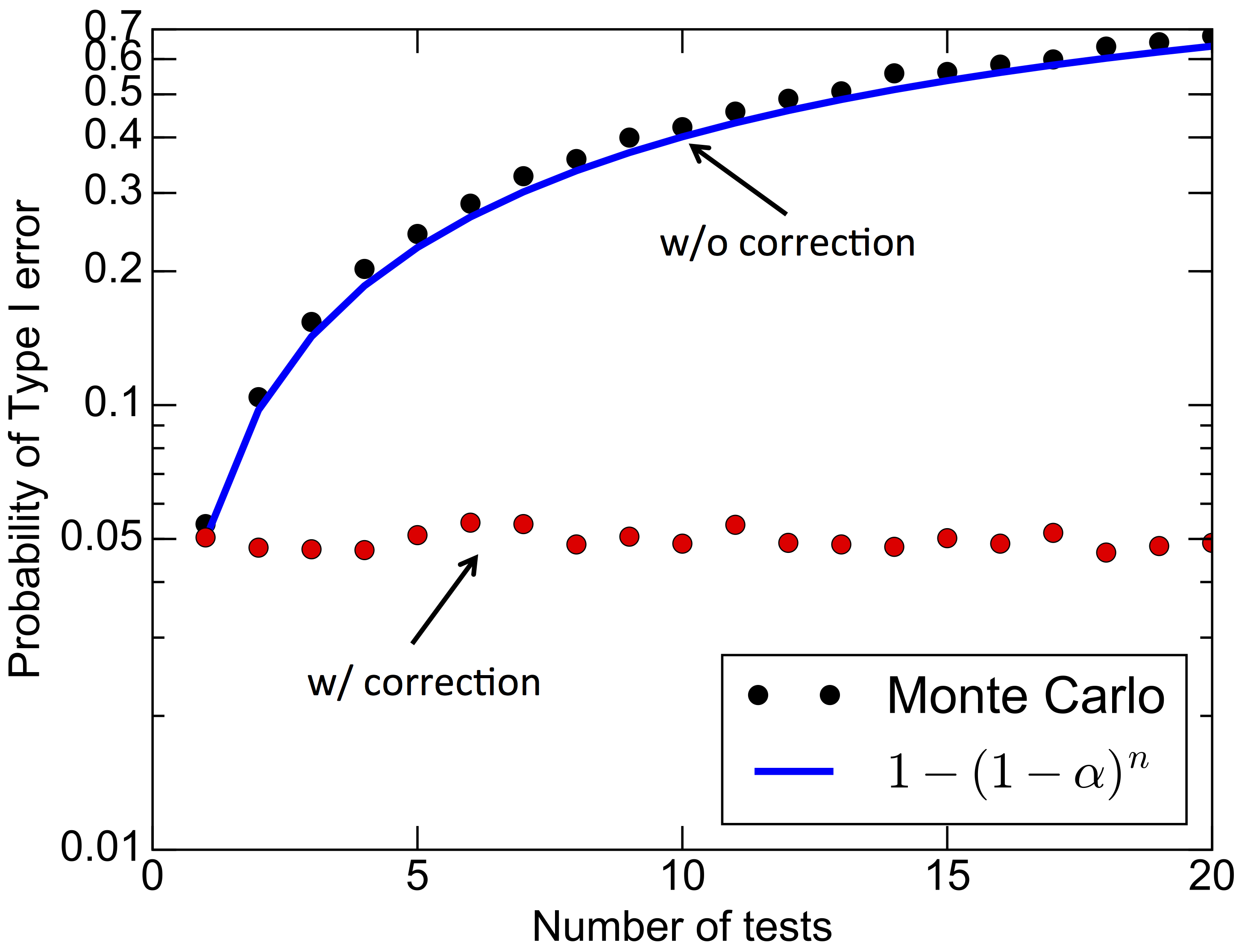
By our definition, the null $H_0$ is true as we are going to set $\mu_A=\mu_B=0.5$ (hence $\Delta \mu=0$). The figure below shows the probability of committing a type-I error as a function of the number of independent t-tests, assuming $\alpha=0.05$. Without correction, the Monte Carlo results are well fitted by eq. (\ref{eq:typeI_independent}) and show a rapid increase of the type-I error rate. Applying the Bonferroni correction does succeed in controlling the error at the nominal 5%.
Below is the Python code that I used to produce the figure above (code that you can also download). The parameter nsims that I used for the figure was 5000, but I had my machine running for a couple of hours so I decided to use 1000 as default. Give it a try, if you are curious!
[download multiple_testing.py ]
1 | import scipy as sp |
⁂