This post is the second one of the series on how to numerically solve 1D parabolic partial differential equations (PDEs). In my previous post I discussed the explicit solution of 1D parabolic PDEs and I have also briefly motivated why it is interesting to study this type of problems.
We have seen how an explicit scheme of solution may require the time step to be constrained to unacceptably low values, in order to guarantee stability of the algorithm.
In this post we will see a different scheme of solution that does not suffer from the same constraint. So let’s go back to the basic equation that we want to solve numerically,
\begin{equation}
\frac{\partial u}{\partial t} = D\frac{\partial^2 u}{\partial x^2} \ + \mathrm{I.B.C.}
\label{eq:diffusion}
\end{equation}
In an explicit scheme of solution we use forward-differencing for the time derivative $\partial u/\partial t$, while the second derivative $\partial^2 u/\partial x^2$ is evaluated at the time step $j$.
In an implicit scheme of solution, we use a different way of differencing eq. (\ref{eq:diffusion}). We still use forward-differencing for the time derivative, but the spatial derivative is now evaluated at the time step $j+1/2$, instead of the time $j$ as before, by taking an average between the time step $j$ and the time step $j+1$,
$$\begin{equation} \frac{\bbox[white,5px,border:2px solid red]{ u_{i,j+1}}-u_{i,j}}{\Delta t} = \frac{u_{i+1,j+1/2}-2u_{i,j+1/2}+u_{i-1,j+1/2}}{\Delta x^2} \\ = \frac{D}{2}\left(\frac{\bbox[white,5px,border:2px solid red]{u_{i+1,j+1}}-2\bbox[white,5px,border:2px solid red]{u_{i,j+1}}+\bbox[white,5px,border:2px solid red]{u_{i-1,j+1}}}{\Delta x^2} + \frac{u_{i+1,j}-2u_{i,j}+u_{i-1,j}}{\Delta x^2} \right). \label{eq:CN} \end{equation}$$Note how the terms inside the red boxes are all unknown, as they are the values at the next time step (the values at the timestep $j$ is instead assumed to be known).
Intuitively, this seems a more precise way of differencing than the explicit scheme since we can now argue that the derivatives on both the left and right hand sides are evaluated at the time $j+1/2$. The scheme of eq. (\ref{eq:CN}) is called Crank-Nicolson after the two mathematicians that proposed it. It is a popular way of solving parabolic equations and it was published shortly after WWII. The Crank-Nicolson scheme has the big advantage of being a stable algorithm of solution, as opposed to the explicit scheme that we have already seen.
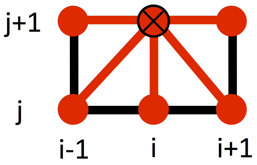
The disadvantage is that it is computationally more difficult to solve eq. (\ref{eq:CN}), as there are now four unknowns in the equation, instead of just one as in the explicit scheme. As the figure below shows, the solution $u(i,j+1)$ depends on quantities already known from the previous iteration, just as in the explicit scheme: $u(i-1,j), u(i,j)$ and $u(i+1,j)$. However, it also depends on quantities at the current iteration: $u(i-1,j+1), u(i,j+1)$ and $u(i+1,j+1)$).
How can we find all the values of the solution $u$ at the time step $j+1$? Since it is not possible to calculate $u(i,j+1)$ directly (explicitly) but only indirectly (implicitly), the Crank-Nicolson scheme belongs to the family of schemes named implicit. The trick is to solve for all the equations $i=2\dots N-1$ (the values at $i=1$ and $i=N$ are known via the boundary conditions) at once. These equations define a linear system, with $N-2$ unknowns in $N-2$ equations.
After rearranging the unknown values to the left and the known values to the right, equation (\ref{eq:CN}) looks like
$$\begin{equation} -r\,u_{i-1,j+1} + (2+2r)u_{i,j+1} -r\,u_{i+1,j+1} = r \,u_{i-1,j} + (2-2r) u_{i,j} + r\,u_{i+1,j}\ , \label{eq:CN1} \end{equation}$$where $r=D\Delta t/\Delta x^2$.
For each inner grid point $i=2,3,\dots N-1$ (as noted, the points at $i=1$ and $i=N$ are supposed to be known from the boundary conditions) there will be an equation of the same form as eq. (\ref{eq:CN1}). The whole set of equations can be rewritten in matrix form as
$$\begin{equation} \left( \begin{matrix} 2+2r & -r & & & \\ -r & 2+2r & -r & \Huge{0} &\\ & & \ddots & & & \\ & \Huge{0} & -r & 2+2r & -r \\ & & & -r & 2+2r \\ \end{matrix} \right) \left( \begin{matrix} u_{2,j+1} \\ u_{3,j+1} \\ \vdots \\ u_{N-2,j+1} \\ u_{N-1,j+1} \\ \end{matrix} \right) = \\ \left( \begin{matrix} 2-2r & r & & & \\ r & 2-2r & r & \Huge{0} &\\ & & \ddots & & & \\ & \Huge{0} & r & 2-2r & r \\ & & & r & 2-2r \\ \end{matrix} \right) \left( \begin{matrix} u_{2,j} \\ u_{3,j} \\ \vdots \\ u_{N-2,j} \\ u_{N-1,j} \\ \end{matrix} \right) + \left( \begin{matrix} r u_{1,j} \\ 0 \\ \vdots \\ 0 \\ r u_{N,j} \\ \end{matrix} \right) \end{equation}$$which can be rewritten as
$$\begin{equation} A\textbf{u}_{j+1} = B\textbf{u}_{j} + \textbf{b}_{j}, \end{equation}$$The definitions of $A, \textbf{u}_{j+1}, \textbf{u}_{j}$ and $\textbf{b}_{j}$should be obvious from the above, but for completion let’s write them down anyways,
$$\begin{equation}
A =
\left(
\begin{matrix}
2+2r & -r & & & \\
-r & 2+2r & -r & \Huge{0} &\\
& & \ddots & & & \\
& \Huge{0} & -r & 2+2r & -r \\
& & & -r & 2+2r \\
\end{matrix}
\right)
,
\textbf{u}_{j+1} =
\left(
\begin{matrix}
u_{2,j+1} \\
u_{3,j+1} \\
\vdots \\
u_{N-2,j+1} \\
u_{N-1,j+1} \\
\end{matrix}
\right)
\\
B = \left(
\begin{matrix}
2-2r & r & & & \\
r & 2-2r & r & \Huge{0} &\\
& & \ddots & & & \\
& \Huge{0} & r & 2-2r & r \\
& & & r & 2-2r \\
\end{matrix}
\right),
\textbf{u}_{j} =
\left(
\begin{matrix}
u_{2,j} \\
u_{3,j} \\
\vdots \\
u_{N-2,j} \\
u_{N-1,j} \\
\end{matrix}
\right),
\textbf{b}_{j}
= \left(
\begin{matrix}
r u_{1,j} \\
0 \\
\vdots \\
0 \\
r u_{N,j} \\
\end{matrix}
\right)
\end{equation}$$
After multiplying both sides by the inverse $A^{-1}$, we find the general solution
$$\begin{equation} \bbox[lightblue,5px,border:2px solid red]{\textbf{u}_{j+1} = A^{-1}B\,\textbf{u}_{j} + A^{-1}\textbf{b}_{j}} \end{equation}$$which needs to be iterated for as many time steps an needed.
Now comes the difficult part: evaluating the stability of the Crank-Nicolson scheme. It can be shown that the matrix $B’:=A^{-1}B$ is symmetric (and real), therefore its 2-norm $||\cdot||_2$ is equivalent to its spectral radius $r(B’)=\max_k |\lambda_k|$, where $\lambda_k$ are the eigenvalues of $B’$,
$$\begin{equation} ||B'||_2 = r(B') = \max_k \left| \frac{1-2r\sin^2k\pi/2N}{1+2r\sin^2k\pi/2N}\right| < 1 \ \ \ \forall \ r>0. \end{equation}$$The result $||B'||_2<1 \ \forall \ r>0$ ensures that the Crank-Nicholson scheme is unconditionally stable, in the sense that the stability condition $||B'||_2<1$ does not depend on the choice of the grid size, time step and diffusion coefficient (parameters that enter in the definition of $r=D\Delta t/\Delta x^2$).
As a final note, it is important to point out that the Crank-Nicolson scheme has a truncation error of $O(\Delta t^2,\Delta x^2)$ as opposed to the explicit scheme that is $O(\Delta t,\Delta x^2)$.
In the next post of this series, I will be looking at a practical implementation of the Crank-Nicolson scheme using Python. That’s it for now, time to look at some computer-generated art…
⁂