Changepoint Detection (CPD) refers to the problem of estimating the time at which the statistical properties of a time series… well… change. It originates in the 1950s, as a method used to automatically detect failures in industrial processes (quality control) and it is currently an active area of research that can boast of having a website on its own.
CPD is a generally interesting problem with lots of potential applications other than quality control, ranging from predicting anomalies in the electricity market (and, more generally, in financial markets) to detecting security attacks in a network system or even detecting electrical activity in the brain. The point is to have an algorithm that can automatically detect changes in the properties of the time series for us to make the appropriate decisions.
Whatever the application, the general framework is always the same: the underlying probability distribution function of the time series is assumed to change at one (or more) moments in time.
Figure 1 shows two examples of how this might work. Suppose we follow the history of visits on a website for 1000 days. In (a), we clearly see that at the 500th day something happens (maybe Google started indexing the website to the top of its search results). After that moment, the number of visits per day is clearly different. However, things are usually not as good as in this example… we may in fact be in the situation (b) of the figure. If I didn’t tell you that there is a changepoint at the 500th day, would you be able to find it?
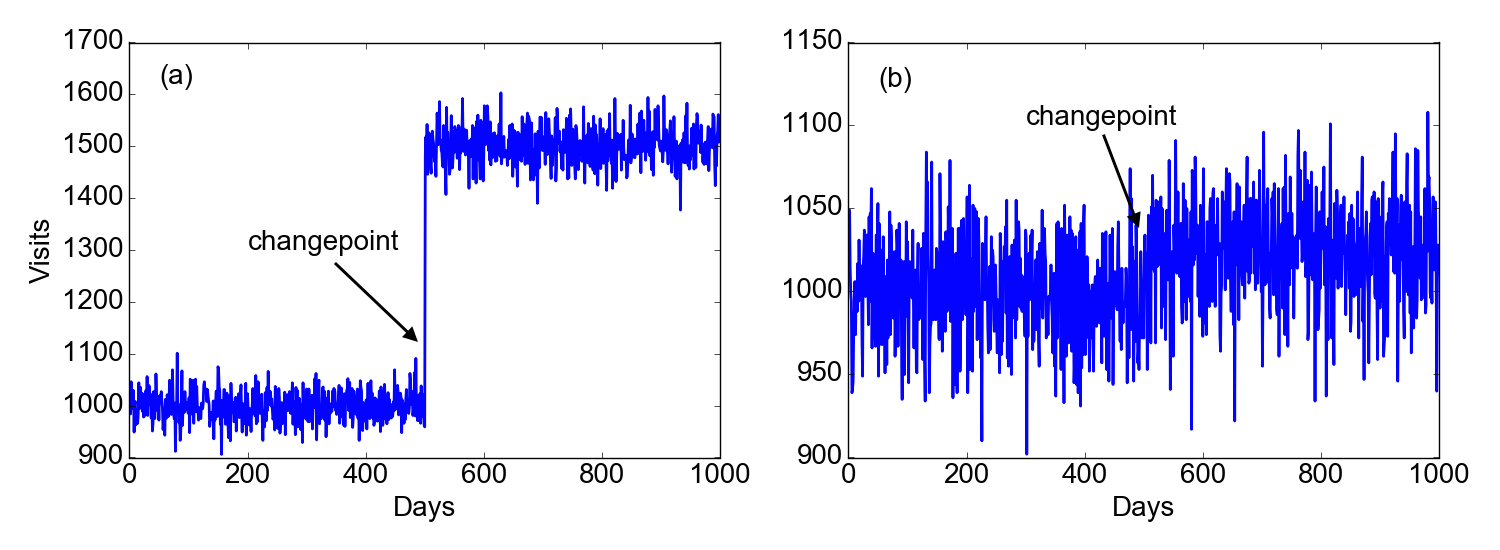 Figure 1. Two time series with a changepoint occurring at Days=500, for an easy (a) and difficult (b) case.
The cases above are examples in which the changepoint occurs because of a change in the mean. In other situations, a changepoint can occur because of a change in the variance, as in the figure below.
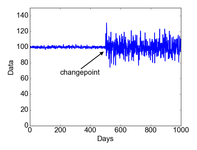 Figure 2. A changepoint can occur because of a change in variance, without necessarily having a change in the mean.
The idea of a CPD algorithm is to being able to automatically detect the positions of the most likely changepoints and, ideally, determine whether there is statistical evidence for claiming them to be “real”.
I will tackle this problem from a frequentist point of view, with the plan of talking about a bayesian approach in a future post.
As in all hypothesis testing problems, there is a potential issue of multiple testing. I have already talked about this issue. To avoid it, I will make the important assumption that the analysis involves a fixed sample so that we are going to perform one single hypothesis test. In other words the analysis is retrospective, as opposed to online sequential in which there is a stream of data that are continuously analyzed.
1. A frequentist solution.
In searching for an R package on CPD, I found changepoint to be very well written and documented. There is a good paper in the Journal of Statistical Software that describes the package in more detail and can be freely accessed here.
In this post I will give my own interpretation on how to approach the problem, although mainly following the arguments and notation of the paper above and of this review.
First of all, for simplicity I will assume that there is a single changepoint during the whole time period, defined at the discrete times t=1,2,3,…,N. This case already captures the essence of CPD.
1.1 Model for a single changepoint
Let’s define τ as the changepoint time that we want to test. Each data point in the time series is assumed to be drawn from some probability distribution function (for example, it could be a binomial or a normal distribution). In this sense, the time series can be considered a realization of a stochastic process. The probability distribution function is assumed to be fully described by the quantity θ (in general, a set of parameters). For example, θ could be the probability p of success in a binomial distribution, or the mean and variance in a normal distribution.
At this point the test goes like this: the null hypothesis is that there is no changepoint, while the alternative hypothesis assumes that there is a changepoint at the time t=τ. More formally, here is our hypothesis test:
H0:θ1=θ2=⋯=θN−1=θNH1:θ1=θ2=⋯=θτ−1=θτ≠θτ+1=θτ+2=⋯=θN−1=θN
The key in the expression H1 above is in the inequality θτ≠θτ+1: at some point in the time series, and precisely between t=τ and t=τ+1, the underlying distribution changes.
The algorithm for detection is based on the log-likelihood ratio. Let’s first define what is the likelihood. The likelihood is nothing else than the probability of observing the data that we have (in the time series), assuming that the null (or the alternative) hypothesis are true. It is a measure of how good the hypothesis is: the highest the likelihood, the higher the data are well fit by the H0 (or H1) assumption.
Assuming independent random variables, under the null hypothesis H0 the likelihood L(H0) is given by the probability of observing the data x=x1,…,xN conditional on H0. In other words,
L(H0)=p(x|H0)=N∏i=1p(xi|θ0)
Let us define the likelihood of the alternative hypothesis,
L(H1)=p(x|H1)=τ∏i=1p(xi|θ1)N∏j=τ+1p(xj|θ2)
The log-likelihood ratio Rτ is then
Rτ=log(LH1LH0)=τ∑i=1logp(xi|θ1)+N∑j=τ+1logp(xj|θ2)−N∑k=1logp(xk|θ0)
Since τ is not known, the previous equation becomes a function of τ. We can thus define a generalized log-likelihood ratio G, which is the maximum of Rτ for all the possible values of τ,
G=max1≤τ≤NRτ
If the null hypothesis is rejected, then the maximum likelihood estimate of the changepoint is the value ˆτ that maximizes the generalized likelihood ratio,
ˆτ=argmax1≤τ≤N Rτ
In general, the null hypothesis is rejected for a sufficiently large value of G. In other words, there is a critical value λ∗ such that H0 is rejected if
2G=2R(ˆτ)>λ∗
The factor 2 is retained to be consistent with the changepoint package.
The problem is how to define this critical value λ∗. The package changepoint has several ways of defining the “penalty” factor λ∗. Going through the R code, I managed to find the definition of a few of them,
- BIC (Bayesian Information Criterion): λ∗=klogn
- MBIC (Modified Bayesian Information Criterion): λ∗=(k+1)logn+log(τ)+log(n−τ+1)
- AIC (Akaike Information Criterion): λ∗=2k
- Hannan-Quinn: λ∗=2klog(logn)
where k is the number of extra parameters that are added as a result of defining a changepoint. For example, it is k=1 if there is just a shift in the mean or a shift in the variance.
At this point we are ready to look into a few more specific examples.
1.2 Normally distributed random variables - change in mean
Assume the variables that compose the time series are drawn from independent normal random distributions. We want to test the hypothesis that there is a change in the mean of the distribution at some discrete point in time τ, while we assume that the variance σ2 does not change. The probability density function is
f(x|μ,σ)=1√2πσ2e−(x−μ)2/2σ2Let us call μ1 the mean before the changepoint, μ2 the mean after the changepoint and μ0 the global mean.
Under the null hypothesis there is no change in mean so the likelihood looks like
LH0=1√2πσ2NN∏i=1exp[−(xi−μ0)22σ2]Under the alternative hypothesis, a changepoint occurs at the time τ and the corresponding likelihood will then be
LH1=1√2πσ2Nτ∏i=1exp[−(xi−μ1)22σ2]N∏j=τ+1exp[−(xj−μ2)22σ2] .Okay, nothing really new so far. Equations (???) and (???) are in fact just specializations of eqs. (???) and (???) to the case of normally distributed random variables.
Now it is time to write the log-likelihood ratio, as in eq. (???), obtaining
Rτ=log(LH1LH0)=−12σ2[τ∑i=1(xi−μ1)2+N∑j=τ+1(xj−μ2)2−N∑k=1(xk−μ0)2]
after which we should calculate G and then apply the criterion (???).
1.3 Normally distributed random variables - change in variance
If there is a change in variance, rather than in mean, the analysis goes pretty similar to the previous section. Let us call y0 and σ20 the global mean and variance, respectively. Under the null hypothesis, the likelihood is
LH0=1√2πσ2N0N∏i=1exp[−(xi−μ0)22σ20]and under the alternative hypothesis,
LH1=1√2πσ2τ1σ2(N−τ)2τ∏i=1exp[−(xi−μ0)22σ21]N∏j=τ+1exp[−(xj−μ0)22σ22] .
The log-likelihood ratio is somewhat more complicated than before,
Rτ=log(LH1LH0)=Nlogσ0−τlogσ1−(N−τ)logσ2+N∑k=1(xk−μ0)22σ20−τ∑i=1(xi−μ0)22σ21−N∑j=τ+1(xj−μ0)22σ22
However, noting that ∑Nk=1(xk−μ0)2=Nσ20, ∑τi=1(xi−μ0)2=τσ21 and ∑Nj=τ+1(xj−μ0)2=(N−τ)σ22 the three last terms in eq. (???) cancel out. The final expression for Rτ is then
1.4 Bernoulli distributed random variables - change in mean
The Bernoulli distribution is possibly the easiest distribution of all. It models binary events that have probability p of happening and probability 1−p of not happening. This is why it is usually introduced in probability theory with the “coin flipping” example.
As before, we can write the likelihood under the null hypothesis
LH0=pm0(1−p0)N−mand under the alternative hypothesis,
LH1=pm11(1−p1)τ−m1pm22(1−p2)N−τ−m2.
The log-likelihood ratio becomes
Rτ=log(LH1LH0)=m1log(p1)+(τ−m1)log(1−p1)+m2log(p2)+(N−τ−m2)log(1−p2)−mlogp0−(N−m)log(1−p0)1.5 Poisson distributed random variables - change in mean
Here we assume that the random variables follow a Poisson distribution,
f(x|λ)=λxe−λx!, x∈N
where x represents the number of events during a pre-defined time interval and λ the expected number of events during the same time interval.
As before, we can write the likelihood under the null hypothesis
LH0=N∏i=1λxi0e−λ0xi!and under the alternative hypothesis,
LH1=τ∏i=1λxi1e−λ1xi!N∏j=τ+1λxj2e−λ2xj!
and the log-likelihood ratio,
Rτ=log(LH1LH0)=τ∑i=1log(λxi1e−λ1xi!)+N∑j=τ+1log(λxj2e−λ2xj!)−N∑k=1log(λxk0e−λ0xk!).
Noting that Nλ0=τλ1+(N−τ−1)λ2, the latter expression can be greatly simplified to give
Rτ=log(LH1LH0)=m1logλ1+m2logλ2−m0logλ0
where m1=∑τi=1xi, m2=∑Nj=τ+1xj and m0=∑Ni=1xk.
2. Applications
We are finally in a position to test the criteria of above for different potential applications. Below I am listing a series of problems with the “solution” underneath. The solution is based on a code that I have written in Python that you can find here,
The code is not optimized, the purpose of it is to show that the methods described above work well at finding single changepoints in time series. The criterion for rejecting (or not) the null is the Bayes Information Criterion (BIC). Feel free to use other criteria.
2.1 Problem 1. Normal distribution: change in mean.
Problem definition: A website receives a certain amount of visits per day. Lately, the marketing team has worked on improving the position of the website on Google searches (Search Engine Optimization). We want to test if this has resulted in an increase in visits on the website.
2.1.1 Parameters of problem 1
Note: these parameters are completely made up. You can change the parameters in the code as you wish, also making the test fail (not rejecting the null),
- Probability density distribution p∼exp[(x−μ)2/2σ2]
- σ=50
- μ=1000 for τ≤2500;μ=1020 for τ>2500
2.1.2 Solution
In IPython, run:
1 | In [1]: run changepoint.py |
 Figure 3. Solution of Problem 1. The Score function is given by eq. (???).
2.2 Problem 2. Normal distribution: change in variance.
Problem definition: Many economists and investors are interested in understanding why financial markets can show abrupt changes in volatility. Assume that such a change in volatility happens in the dataset we are provided. We need to detect when this change happens in the dataset in order to improve our investment model.
2.2.1 Parameters of problem 2
Note: these parameters are completely made up. You can change the parameters in the code as you wish, also making the test fail (not rejecting the null),
- Probability density distribution p∼exp[(x−μ)2/2σ2]
- μ=1000
- σ=10 for τ≤2500;σ=20 for τ>2500
2.2.2 Solution
In IPython, run:
1 | In [1]: run changepoint.py |
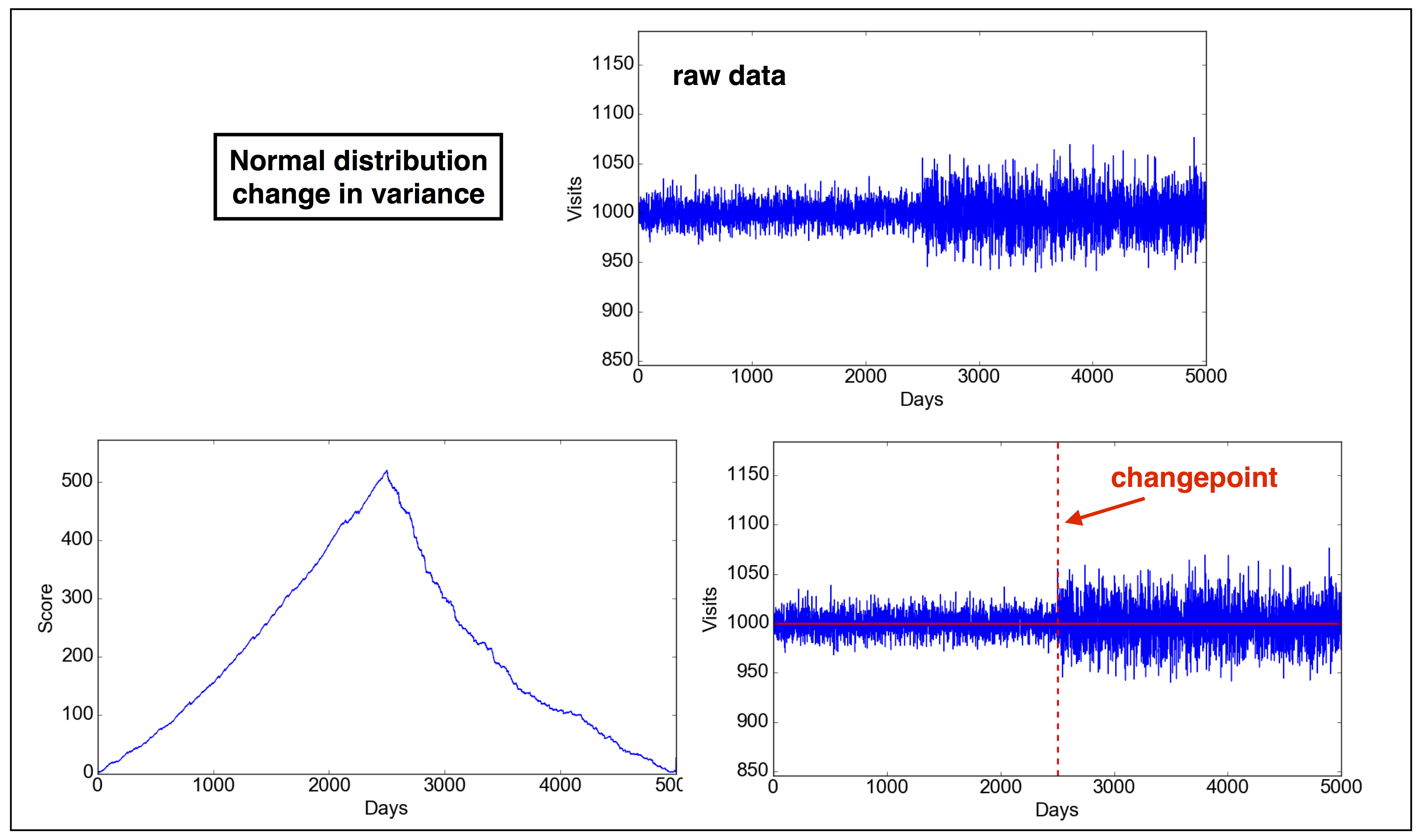 Figure 4. Solution of Problem 2. The Score function is given by eq. (???).
2.3 Problem 3. Bernoulli distribution: change in mean.
Problem definition: An industrial chain delivers products that need to be manually inspected. Under normal circumstances, about 10% of the products are found with small imperfections that need to taken care of. Recently, a potential bug in the software has been found which may have caused an increase in the inspection failure rate. We want to detect when the bug was introduced and whether the failure rate has increased because of it.
2.3.1 Parameters of problem 3
Note: these parameters are completely made up. You can change the parameters in the code as you wish, also making the test fail (not rejecting the null),
- Probability density distribution: inspection fails with probability p, does not fail with probability 1−p
- p=0.10 for τ≤2500;p=0.15 for τ>2500
2.3.2 Solution
In IPython, run:
1 | In [1]: run changepoint.py |
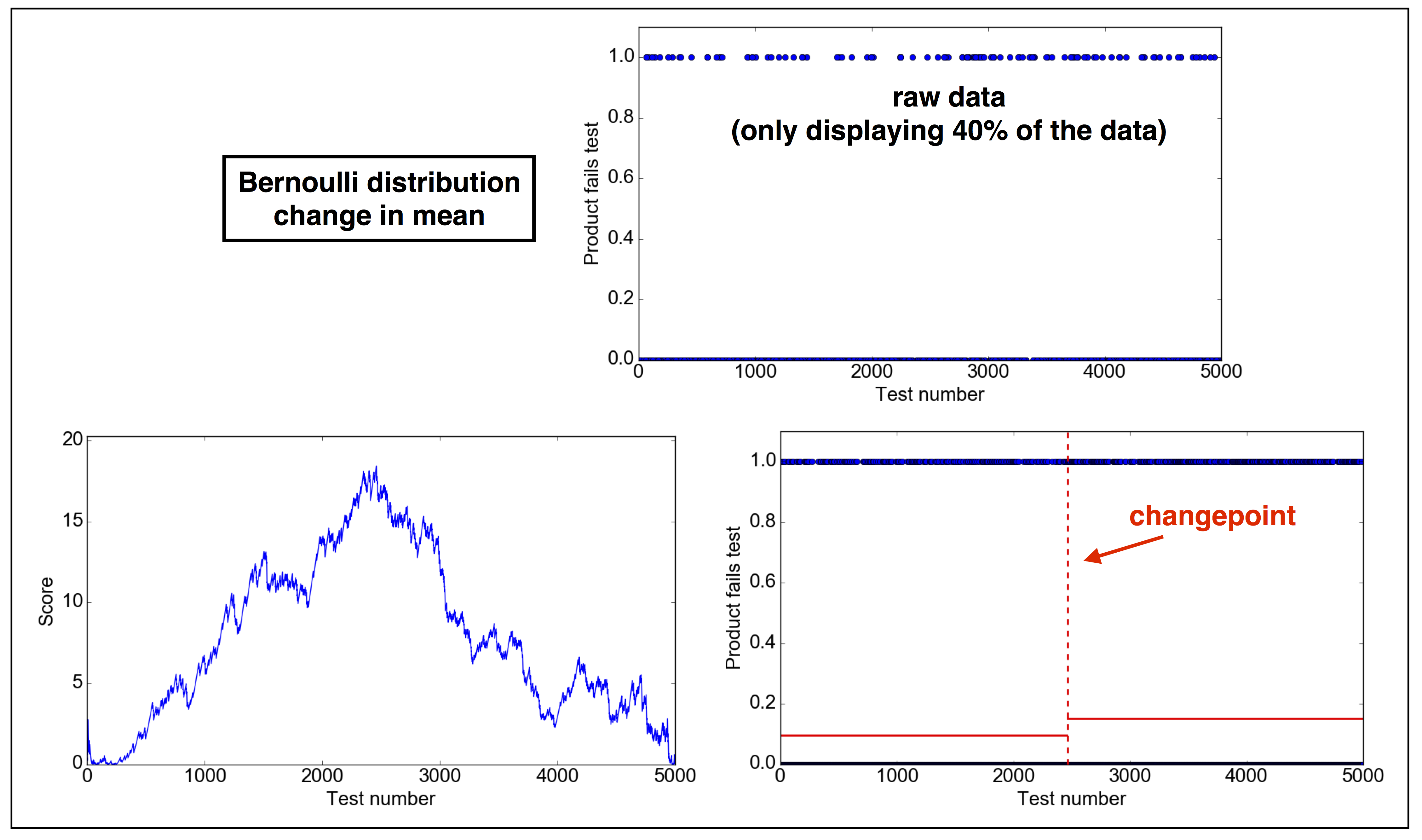 Figure 5. Solution of Problem 3. The Score function is given by eq. (???).
2.4 Problem 4. Poisson distribution: change in mean.
Problem definition: Under normal circumstances, a network system has a load of a few tens of hits per minute. Check whether there is a sudden change in the number of hits per minute in the data provided.
2.4.1 Parameters of problem 4
Note: these parameters are completely made up. You can change the parameters in the code as you wish, also making the test fail (not rejecting the null),
- Probability density distribution: p(k)∼λke−k/k! where k is the observed number of hits per minute and λ is the expected number of hits per minute.
- λ=0.12 for τ≤2500;λ=0.10 for τ>2500
2.4.2 Solution
In IPython, run:
1 | In [1]: run changepoint.py |
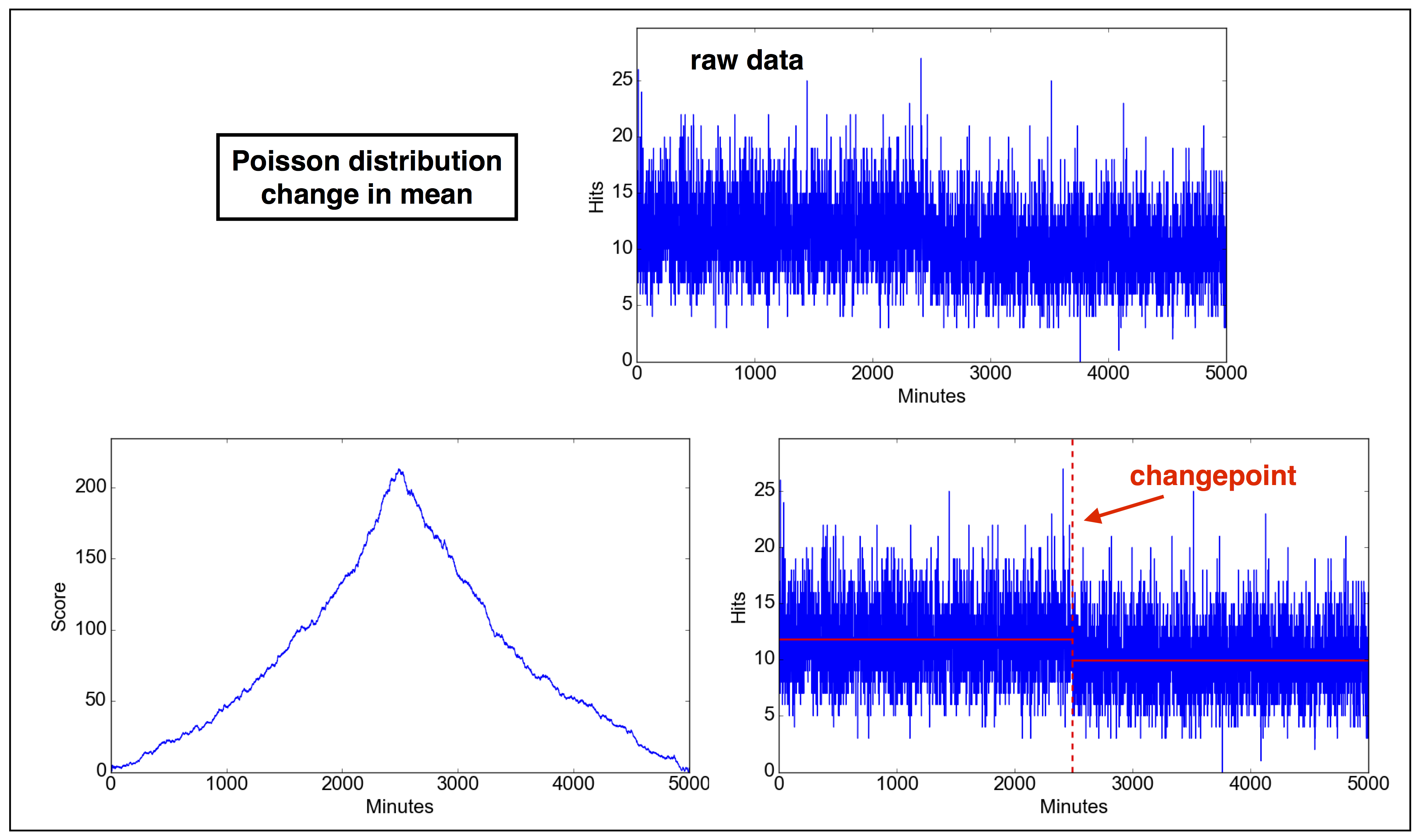 Figure 6. Solution of Problem 4. The Score function is given by eq. (???).
⁂